II Training and Event Considerations

6

Physiological Assessment of Middle- and Long-Distance Runners

Andy Galbraith

Highlights

• • Assessment options exist for the physiological evaluation of a wide range of laboratory and field-based parameters.
• • Laboratory-based physiological assessment should include maximal oxygen uptake (F0_2lMX), running economy (RE), lactate threshold (LT) and the velocity associated with V0_2aax (v-V0_2mJ.
• • Field-based physiological assessment should include critical speed (CS), the maximum distance that can be achieved at speeds above critical speed (D’) and the anaerobic speed reserve (ASR).
• • This test battery covers the key determinants which explain differences between athletes in distance running performance.

Introduction

Within medical terminology, a physiological assessment refers to examination into the functioning state of the human body. It follows therefore, that within exercise science terminology, a physiological assessment can be defined as investigation into how the body’s various physiological systems respond and adapt to exercise. Following on from Chapter 1, the objectives of this chapter are to describe a battery of valid tests that assess the main physiological determinants of middle- and long-distance running performance, provide reference values for interpretation of test results, and outline how test data can be used to inform training prescription.

Purpose and Benefits

The endeavour for continued performance improvement by athletes highlights the need to recognise mechanisms to optimise athletes’ training. Whilst physiological assessments may be conducted for a variety of reasons, a commonly cited rationale for their use includes providing an evaluation of strengths and weakness of the athlete. Such information can then inform training program design, including prescription of individualised optimal training intensities.

Physiological assessment of an athlete may also be useful to monitor and assess the effectiveness of training programmes to understand whether performance is improving, and the associated physiological adaptations are occurring. It has also been suggested an additional benefit of physiological testing for an athlete is that the prospect of regular testing, built into their schedule, may often act as a further motivational influence during a training cycle.

Repeatability of Measures

For data gleaned from physiological testing to be of value to the athlete and coach, it is important that the tests chosen to form part of such assessments are reproducible. This necessitates understanding the extent to which an apparent change in a measure is meaningful and does not lie within the confidence interval for error (Atkinson and Nevill, 1998). Variability in measures of performance can be attributed to technical and biological sources. Technical sources refer to the precision of the instruments utilised, combined with the ability of the tester to operate the equipment efficiently. Biological sources of error within performance tests include cyclic biological variation and motivational changes, which may contribute to small day-to-day variations in test performance of an athlete (Atkinson and Nevill, 1998). A clear understanding of the repeatability of a performance test is important prior to data interpretation. Changes in physiological measures over time may often be small, particularly when working with highly trained athletes; therefore, it is important that a performance test is both sensitive and repeatable, in order to ensure small changes in performance are not masked.

Pre-Test Considerations

In order to minimise the impact of biological sources of error within a performance test, a consistent pre-test routine is important prior to all repeat visits. Where possible, athletes should standardise the time and type of training sessions within the preceding 24 hours of a performance test. Ideally, training within this timeframe should be light recovery-type training. Athletes should avoid fundamental changes to their diet in the days prior to testing and are typically advised to eat no food in the 3 hours before a test. However, it is important that athletes consume adequate fluid in the 12 hours prior to testing. Footwear becomes an important consideration when working with middle- and long-distance runners. Shoes of varying mass may influence the economy of the athlete, therefore influencing the oxygen cost during running (Fuller et al., 2015). Consequently, athletes should be advised to wear the same (or similar) type of shoe for each test session. Environmental conditions should be recorded, with the aim of standardising (as much as possible) conditions across repeat test visits. Finally, an athlete’s familiarisation with the test protocols will influence the repeatability of their performance. Therefore, one or more familiarisation sessions should be considered prior to recording test performances.

Laboratory-Based Testing

When conducting a physiological assessment for an athlete, laboratory-based testing provides the opportunity to ensure a greater level of precision. Environmental conditions can be controlled and replicated, whilst calibrated treadmills offer a consistent velocity at each visit. Consequently, the repeatability of laboratory-based physiological assessments has the potential to be high, increasing the sensitivity of such tests to detect small changes in an athlete’s performance. However, physiological assessment in a laboratory setting takes place in an environment unfamiliar to most athletes.

Field-Based Testing

For the purpose of this chapter, field testing is defined as tests conducted outside the laboratory environment and do not require specialised equipment for data collection or recording (Maud and Foster, 2006). Physiological assessments should endeavour to closely replicate the athlete’s typical exercise conditions. Consequently, field testing is often described as having a higher level of ecological validity than laboratory-based testing (Galbraith et al., 2011). Accordingly, physiological testing conducted in the field may help bridge the gap between the sport scientist, athlete and coach, where field-test protocols better reflect conditions which athletes experience during training and competition (Foster et al., 2006). It has also been suggested that as field testing occurs in the athlete’s natural training/competition environment, the sense of‘missing out’ on training, by participating in the physiological test, may be reduced. Notwithstanding these advantages, field testing creates distinctive challenges for the sport scientist.

Frequency of Testing

Typically, repeat physiological assessments with middle- and long-distance runners would be scheduled approximately every 3 months, typically around October, January, April and July, to correspond with key transitions in an athlete’s seasonal training and competition schedule (Jones, 1998; Galbraith et al., 2014a). However, with the development of field-based test protocols, there is the opportunity for more frequent test points within a training cycle.

Laboratory-Based Physiological Assessment

Assessment options exist for a wide range of laboratory-based physiological parameters which influence middle- and long-distance running performance. This section will focus on three key determinants which have been shown to explain differences between athletes in distance running performance; Maximal oxygen uptake (FO^,^), running economy (RE), and lactate threshold (LT). F0_2lmx characterises an individual’s maximal rate of aerobic energy expenditure (Jones and Carter, 2000). RE describes the oxygen uptake or energy' expenditure required at a given absolute exercise intensity, for example the oxygen uptake required for an athlete to run at 16 km-h The function of V0_2lmx and RE generates the velocity associated with F0_2llMX (v-F0_2max) LT is a parameter with numerous definitions attached to it, which can present some confusion for the scientific and endurance running communities. In its simplest terms, LT is defined here as the exercise intensity corresponding to the first increase in blood lactate above resting levels (Jones and Carter, 2000).

Assessment Techniques (V0_2max, RE, LT, v-V0_2max)

This chapter adopts the treadmill protocol described by Jones (2006b), which has been used to monitor highly trained middle- and long-distance runners (Jones, 1998, 2006b; Galbraith et al., 2014a). This test has the advantage of enabling the measurement and recording of FOjmaxj RE, LT and v-F0_2niax within the same test protocol.

Athletes should be allowed time to complete a self-selected warm-up, which should closely replicate the warm-up routine they use before a typical training session. Prior to the test, the athlete’s body mass and stature should be recorded, along with a fingertip capillary blood sample, to determine resting blood lactate concentration.

The treadmill test is administered in two parts:

Sub-maximal test: the first part is a sub-maximal test, using a treadmill gradient of 1% (Jones and Doust, 1996). The initial treadmill belt speed for this phase of the test should be decided individually for each athlete, based on their current fitness level, with the aim of completing 5 to 9 stages during the sub-maximal phase of the test. Typically, the penultimate phase of the test usually equates to a velocity equivalent to that which the athlete can hold during a 60 min hard run. Therefore, the velocity of the penultimate stage may be close to 10-mile or half-marathon race pace, depending on the ability of the athlete. Each stage of the test should be 4 min in duration; however, with highly trained athletes it has been suggested that 3-min stages are appropriate, due to a faster time to achieve a steady state of oxygen consumption within each stage (Jones, 2006a). The treadmill belt speed should be increased by 1.0 knrlr¹ at the end of each stage; however, for an increased sensitivity of LT determination, 0.5 kmh ¹ increments may be appropriate (Jones, 2006a). Average heart rate during the final 30 seconds of each stage should be recorded. At the end of each 4-min stage, a capillary blood is collected and, if required, perceived level of exertion using the Borg 6-to-20 scale (Borg, 1998). The sub-maximal test should be terminated when a second breakpoint in blood lactate has been observed (see the interpretation section that follows). Typically, once the participant’s blood lactate concentration has normally exceeded 4.0 mmol L^-1, this will have been achieved. Throughout the test, continuous breath-by-breath measurement of the athlete’s expired gases should be collected. An active recovery in the region of 10-15 min should follow the termination of the sub-maximal test, prior to the athlete continuing into the second phase of the treadmill test.

Maximal test: the second phase of the test is used to determine F0_2lmx and the velocity at F0_2max (y-V0_2mJ. This test should be started at a 1% gradient and a velocity 2.0 km h^-1 below the velocity at which the participant finished the first phase of the test. The treadmill velocity should remain constant throughout this phase of the test, with the treadmill gradient increased by 1% ever)' minute until the participant reaches volitional exhaustion. Throughout the test, continuous breath-by-breath measurement of the athlete’s expired gases should be collected, and upon test termination, maximum heart rate recorded.

Maximal Oxygen Uptake (V0_2maJ Interpretation of Test Results and Normative Data

Several methods have been suggested for the calculation of F0_2lmx. However, when utilising breath-by-breath expired air analysis, a simple method is to report the highest F0₂ achieved during the test, using a rolling 1-min average (Galbraith et al., 2014a).

Absolute values for F0_2mlx are reported in units of Lanin however as measures of performance are influenced by the size of the body, a scaled adjustment of the absolute value is common. Traditionally, F0_2lmx is scaled to whole body mass in units of mL kg ' min *, providing a useful method for comparison of F0_2max between different athletes. However, a meta-analysis by Lolli et al. (2017) provided evidence against the normalisation of F0_2max to whole body mass and highlighted the validity of normalising to fat-free mass.

An athlete’s F0_2max score from the treadmill test can be compared to normative data for V0_2max, such as those presented in Table 6.1. This can provide an indication of strengths or weakness within this area, which may then inform future training program design. During repeat assessments, an athlete’s F0_2max score from the treadmill test can be compared to previous scores from the same athlete, providing a useful method to monitor the effectiveness of training programmes and assess whether any adaptation to F0_2max is occurring.

Application of Test Data

In highly trained runners, it has been suggested that K0_2max will eventually stabilise, with any further performance improvements, attributed to sustained development of RE and LT. For example, Billat et al. (1999) reported no change in F0_2max, following a 9-week period of endurance training, in a group of highly trained distance runners (mean F0_2max >

TABLE 6.1 Normative data for F0_2max (mLkg '-min ') for male and female distance runners

Note: Values are based on data collected from highly trained runners.

70 mL-kg^-1-min^-1). Furthermore, Martin et al. (1986) evaluated nine highly trained male distance runners (mean F0_2lmx > 70 mL-kg^-1-min^-1) over a 30-month period, during their preparation for Olympic trials. Across ten repeat treadmill tests, data highlighted no significant change in F0_2max during this monitoring period, whilst anaerobic threshold increased by 5.6%. In addition, Jones (1998) report no increase in F0_2max (actually a slight decrease) across a 5-year monitoring period in a world-class female distance runner. However, in contrast Galbraith et al. (2014a) reported a ~5% increase in V0_2max following a 1-year period of endurance training in highly trained distance runners (mean F0_2max > 70 mL-kg ' tnin ^_1). In recreationally trained athletes, F0_2max improvements of 5-10% have been observed following a 6-week programme (Franch et al., 1998; Carter et al., 1999).

Londeree (1986) used data from elite middle- and long-distance runners to estimate the percentage of F0_2max that can be maintained for various periods of time. Using these data, it can be estimated that, in highly trained athletes, an 800 m race will require the energetic equivalent of~120% F0_2max, the 1500 m ~ 110% F0_2max, 5000 m ~96% F0_2lmx, 10,000 m ~92% F0_2max and the marathon ~ 85% FO,_max (Jones, 2006a). Whilst F0_2max is an important determinant of success for all distance running events, these data highlight that as the competitive distance increases, sub-maximal physiological measures, such as RE and LT, may increase in importance.

Running Economy

Interpretation of Test Results and Normative Data

Reporting the oxygen cost from the treadmill test at a set speed may not provide a fair comparison across athletes of different ages and abilities, therefore it may be useful that RE is calculated over the range of sub-maximal velocities used during the first phase of the treadmill test, by recording the average V0₂ (mL-kg^-1-min^-1) for the last minute of each steady-state stage (Galbraith et al., 2014a). Alternatively, reporting the RE at LT speed may provide usefiil comparisons. Barnes and Kilding (2015a) provide comprehensive normative running economy data for male and female runners of varying ability levels. According to these data:

Recreationally trained runners at 12 km-h^-1 report a mean RE of 42.2 mL-kg '-min^-1 (range 40.4-45.3) for males and a mean of 43.2 mL-kg^-1-min^-1 (range 38.5-48.1) for females.

Moderately trained runners at 14 km-h^-1 report a mean RE of 46.8 mL-kg '-min^-1 (range 42.0-55.5) for males and a mean of 47.9 mL-kg^-1-min^-1 (range 41.3-53.5) for females.

Highly trained runners at 16 km-h^-1 report a mean RE of 50.6 mL-kg^-,-min^-1 (range 40.5—66.8) for males and a mean of 54.5 mL-kg^-1-min^-1 (range 46.2-61.9) for females.

RE can also be reported in units of mL-kg ' km^-1, by inputting the average FD₂at the chosen intensity into the following equation (Jones, 2006a):

Normative data for RE in these measurement units have been reported by Jones (2006a) as:

Excellent: 170-180 mL-kg^-,-km^-1

Very Good: 180-190 mL-kg^-,-km^-1

Above Average: 190-200 mL-kg^-,-km^-1 Below Average: 200-210 mL-kg^_,-km^_1 Poor: 210-220 mL-kg^-,-km^-1

Finally, RE can be presented as the energy cost of running (rather than the oxygen cost), reported in units of kcal-kg^-1-km^-1 or kj-kg^_1-km^_1. Shaw et al. (2014) suggest this provides a more valid index of RE and suggest using the updated nonprotein respiratory quotient equations of Peronnet and Massicotte (1991) to estimate substrate use (g.min^-1) during the final minute of each stage. Subsequently, the energy derived from each substrate can be calculated by multiplying fat and carbohydrate usage by 9.75 (40.81) and 4.07 (17.04) kcal (kj) respectively and presenting RE as the sum of these values, expressed in kcal-kg^-1-km^-1 or kJ-kg-’-km^-1.

Normative data for RE reported in kcal-kg^-1-km^-1 are provided by Shaw et al. (2014) who reported data from a sample of 172 highly trained male and female middle/long-distance runners. Data were reported across four speeds ranging from 12.4 to 15.4 km-lf¹'¹ for females and 13.8 to 16.8 km-lf¹ for males. RE increased at each speed, with mean values ranging from —1.14 to 1.18 kcabkg '-km ¹ (4.77 to 4.94 k|-kg^_1-km^_l) on average across the four speeds for the subject group. Similar data have been reported by Galbraith et al. (2014a) in a group of highly trained male athletes, with RE values between 1.13 and 1.17 kcal-kg^_l-km^_l (4.73-4.94 kJ-kg-'-knT¹).

Scaling of RE data to an exponent of body mass (BM) is common, with a comprehensive analysis of 172 distance runners by Shaw et al. (2014), reporting that linear scaling of RE to BM"¹ appeared to be the most appropriate method to remove the influence of body mass on RE in endurance runners.

Application of Test Data

The degree of change in RE following a period of endurance training will depend on the initial fitness level of the individual, with greater scope for a higher magnitude improvement in less highly trained individuals. However high magnitude improvements in RE, following a longitudinal period of endurance training, have still been reported in highly trained individuals, with Jones (1998) reporting a gradual improvement of RE across a 5-year period in a highly trained female distance runner, with values improving from ~200 lnL-kg ' -kin ¹ to ~180 mL-kg '-km '. The majority of research investigating changes in RE following training has been conducted over relatively short durations (~6-8 weeks). Where already trained runners are concerned, a short period of ‘normal’ endurance training appears to have little effect on RE (Paavolainen et al., 1999a; Spurrs et al., 2003; Johnston et al., 1997; Turner et al., 2003). However, improvements in running economy can sometimes be observed with short-term training programmes in less-trained individuals. In a recent study, Jones et al. (1999) reported that a 6-week endurance training programme, consisting of continuous and interval running at a speed close to LT, caused a significant improvement in running economy- in recreationally active students, with values improving from —195 mL-kg '-km ¹ to ~180 mL-kg'-knr¹. In already-trained runners, it would appear that an additional stimulus above that of typical training is needed in order to generate a short-term improvement in RE. The addition of high-intensity interval running training demonstrated improvements of ~3-7% in RE over the course of a 6- to 8-week training period (Billat et al., 1999; Laffite et al., 2003; Franch et al., 1998; Yoshida et al., 1990). Whilst the addition of explosive strength/plyometric training has been shown to produce ~2-7% improvement in RE across a 6- to 9-week training period (Paavolainen et al., 1999a; Spurrs et al., 2003; Turner et al., 2003).

An improvement in RE will result in the utilisation of a lower percentage of F0_2max for any given exercise intensity. To put this into context, an athlete with a F0_2lmx of 70 mL-kg^-1-min^-1, who displays a RE of 200 mL-kg^-1-km^-1 whilst running at 16 km-h^-1, would be working at 76% of their F0_2max. A 5% improvement in RE, following a training intervention, would mean the athlete was now only using 72% of their F0_2max to run at the same speed. Further, as oxygen consumption is directly related to energy expenditure, the athlete would require less energy to run at this speed, preserving energy for later in the race.

Velocity at Maximal Oxygen Uptake (v-V0_2maJ Interpretation of Test Results and Normative Data

v-F0_2max describes the relationship between V0₂ at a sub-maximal exercise intensity and F0_2imx and is calculated by solving the regression describing this relationship (Jones, 1998). A simple equation to allow the estimation of v-F0_2max from the previously described treadmill test was provided by Jones (2006a):

Where F0_2max (mL kg '-imn ') is calculated as highest F0₂ achieved during the maximal phase of the treadmill test, using a rolling 1-minute average. Whilst RE (mL-kg^-1-km^-1) is taken as the average F0₂ achieved during the last minute of each stage of the sub-maximal phase of the treadmill test (taken as an average of this value over the first 4-5 stages). Using the example athlete described in the previous section, who reported with a F0_2max of 70 mL-kg'-min^-1 and a RE of 200 mL-kg ' km⁴, the corresponding v-F0_2maxfor this athlete can be estimated at 21.0 km-h^-1.

Normative data for v-V0_2max from a cohort of highly trained (mean F0_2max > 70 mL-kg^-1-min^-1) male middle- and long-distance runners were presented by Galbraith et al. (2014a) with values ~19—20 km-h^-1 across repeat tests over a training year. This is supported by the data from Billat et al. (1999), who report a mean v-F0_2max of 21.1 ± 0.8 km-h^-1 in a small group of highly trained (F0_2max ~72 mL-kg^-1 min^-1) male middle- and long-distance athletes. In female athletes, Jones (1998) reports a peak v-F0_2max of 20.4 km-h^-1 during a 5-year case study of a world-class female distance runner. Whilst in recreational athletes, Jones et al. (1999) report values in the region of~15-17 km-h^-1 in a group of sports students.

Application of Test Data

v-F0_2max has been reported as a strong predictor of distance running performance (Morgan et al., 1989a; Jones and Doust, 1998; Jones, 1998), with particular relevance in middle-distance events (Jones and Carter, 2000). Additionally, it has been suggested that the v-FD_2max

provides an optimal speed to train at to stimulate improvements in F0_2lmx. Training-induced improvements in v-F0_2max will result in a given percentage of K0_2max being associated with a faster running speed. Therefore, as a 3000 m race, for example, requires an athlete to run at ~100% of their F0_2max (Londeree, 1986; Jones, 2006a), the link between an improvement in v- K0_2mix and an increase in race speed becomes apparent. In a purely mathematical example, an increase in v-F0_2nuxfrom 19.0 to 19.2 kmlf¹ (1% improvement) would lead to a theoretical improvement of~5 seconds in 3000 m time. The degree of change in v-F0_2max following a period of endurance training will depend on the initial fitness level of the individual, with greater scope for a higher magnitude improvement in less highly trained individuals. Improvements of ~3-7% have been reported for short- and long-term training programmes respectively, in highly trained athletes (Jones, 1998; Billat et al., 1999). In more recreationally trained athletes, Jones et al. (1999) reported a ~9% increase following a 6-week period of training.

Lactate Threshold

Interpretation of Test Results and Normative Data

LT is a parameter with numerous definitions attached to it, which can present some confusion for the scientific and athletic sporting communities. In a review of research within this area, Faude et al. (2009) identified 25 different LT concepts within published literature. Two thresholds (breakpoints) are commonly used (Figure 6.1), which in theory can be identified from a plot of the blood lactate (y axis) against running speed (x axis) data, obtained during the sub-maximal phase of the treadmill test. Flowever, in practice this can prove problematic, with differences in the LT values identified via these methods, reported across different observers (Yeh et al., 1983).

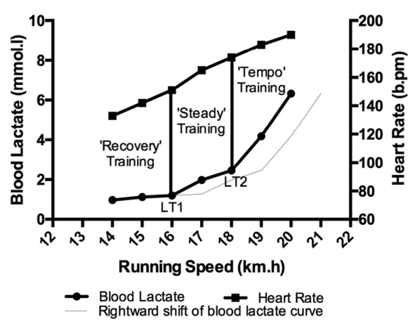
FIGURE 6.1 Example blood lactate and heart rate data from the sub-maximal treadmill test

Lactate threshold: In its simplest terms, the 1st LT (or aerobic threshold) (LT1 on Figure 6.1) is defined as the exercise intensity (running speed) corresponding to the first increase in blood lactate above baseline levels (Jones and Carter, 2000; Jones, 2006a). In an effort to add a level of objectivity to the assessment, LT is often defined as the exercise intensity associated with a fixed blood lactate level, such as 2 mmol-L^-1, or identified as the exercise intensity that produces a fixed increase in blood lactate above baseline values, for example a 1 mmol-L ¹ increase in blood lactate concentration above baseline (Hagberg and Coyle, 1983).

Maximal steady state: The 2nd LT (or anaerobic threshold) (LT2 on Figure 6.1) has been defined as the running speed at which a sudden and sustained increase in blood lactate is observed (Smith and Jones, 2001; Jones, 2006a). This point will sit somewhere between LT1 and F0_2nlax and is identified as the second breakpoint seen when plotting the blood lactate vs. running speed relationship (identified as LT2 on Figure 6.1). A fixed blood lactate level of 4 mmol-L^-1 is also often implemented to identify this threshold. A further frequently used method of identifying this threshold is the D_max concept, with Jamnick et al. (2018) reporting a modified D_max method as the most valid estimate of maximal steady state.

The exercise intensity at LT is typically reported as a running speed (km-h^-1) or a running pace (mimmile or min:km). In addition, it is useful to also report the heart rate in beats per minute (b-min '*) required to exercise at this speed/pace. Due to the numerous different concepts used in the literature to describe LT, presenting normative data is problematic for this parameter. Normative data for LT1 (1 mmol above baseline) from a cohort of highly trained (mean F0_2max> 70 mL-kg^-1-min^-1) male middle- and long-distance runners were presented by Galbraith et al. (2014a) with values averaging 15.7 ±1.2 km-h^-1 (6:09 min:mile) across repeat tests over a training year. In female athletes, Jones (1998) reports LT (a clear threshold increase in blood lactate from a plot of blood lactate against running speed) values ranging from 15.0 (6:26 mimmile) to 18.0 km-h ¹ (5:22 mimmile) during a 5-year case study of a world-class female distance runner. Whilst in recreational athletes, Jones et al. (1999) report values for LT (a clear threshold increase in blood lactate from a plot of blood lactate against running speed) of 11.2 ± 1.8 km-h ¹ (8:37 mimmile) in a group of sports students. In a group of trained (mean K0_2lmx 65.9 ± 4.2 mL-kg^-l-min^-1) male junior-distance runners, Tanaka et al. (1984) report values for LT (a marked increase above baseline values) at 14.7 ± 1.4 km-h^-1 (6:34 mimmile). Finally, Billat et al. (1999) present data for LT2 (velocity at OBLA), at 17.6 ± 1.0 km-h^-1 in a small group of highly trained (FD_2max ~72 ml-kg^-l-min^-1) male middle- and long-distance athletes.

Application of Test Data

A rightward shift of the LT to a higher running speed is characteristic ofsuccessfi.il endurance training programmes. This rightward shift of the blood lactate vs. running speed relationship (pale dotted line on Figure 6.1) allows a faster running speed to be sustained at a given blood lactate level (Jones and Carter, 2000).

The degree of change in LT following a period of endurance training will depend on the initial fitness level of the individual, with greater scope for a higher magnitude improvement in less highly trained individuals. However, high magnitude improvements in LT1, following a longitudinal period of endurance training, have still been reported in highly-trained individuals, with Jones (1998) reporting a 20% improvement in LT1 during a 5-year monitoring period in a world-class female distance runner. In contrast, Galbraith et al. (2014a) report little variation (<1%) in LT1 over the course of a training year, in a group of highly trained (mean F0_2max >70 mL-kg^-1-min^-1) male middle- and long-distance runners. However, in a group of trained (mean K0_2nux 65.9±4.2 mL-kg^_1-min^_l) male junior distance runners, Tanaka et al. (1984) report a ~2% increase in LT1 from pre- to post-season. In more recre- ationally trained athletes, Jones et al. (1999) report a ~6.5% increase in LT, following a 6-week period of continuous and interval running training in a group of sports students (F0_2max ~50 mL kg^_1min^_l). Training-induced improvements in LT2 (maximum steady state) have also been reported. In a small group of highly trained (F0_2lmx ~72 mL-kg '-mm ') male middle- and long-distance athletes, Billat et al. (1999) report a ~2.5% increase in LT2 (maximum steady state) following a short-term (4-week) training programme, involving interval sessions based around the v-F0_2max.

Jones (2006a) suggest that the speed at LT 1 is closely related to the speed that can be sustained over a marathon, whilst the speed at LT2 (maximum steady state) can be maintained for ~60 min in highly trained runners, so it may be closely related to the speed that can be sustained over 10 miles to half-marathon distances (Jones, 2006a).

LT data from the treadmill test also have a useful application in the design of training sessions for athletes. The speed at LT and the heart rate associated with this speed are useful in demarcating transition points between the various exercise intensity zones (Figure 6.1). For example, speeds/heart rates below LT1 may provide useful intensities for easy or ‘recovery’ training runs. The speeds/heart rates between LT1 and LT2 (maximum steady state) may provide useful intensities for ‘steady’ running sessions, whilst the speeds/heart rates above LT2 (maximum steady state) may provide useful intensities for training runs set at a more ‘tempo’ pace (Jones, 2006a).

Training at the LT provides an aerobic training stimulus, whilst enabling blood lactate levels to remain low, allowing high millage runs to be conducted at this intensity. In general, it appears that training at intensities close to or slightly above the LT are important for stimulating improvements in the LT (Carter et al., 1999).

Field-Based Physiological Assessment

Field-based assessment protocols aim to closely replicate the athlete’s typical exercise conditions, affording field tests a high level of ecological validity (Galbraith et al., 2011). Field-based assessment, therefore, provides a useful alternative (or enhancement) to laboratory-based testing, when conducting physiological assessment for middle- and long-distance runners. Research describing valid and reliable assessment methods for field-based testing are less prevalent in the scientific literature, but such research has been increasing in popularity in recent years. This section will focus on three key physiological parameters, which can form part of a fitness-testing battery, when working with middle- and long-distance runners: critical speed, D’ and the anaerobic speed reserve. A runner’s critical speed (CS) has been suggested to reflect the highest sustainable running speed that can be maintained without a continual rise in V0₂ to F0_2max, whilst D’ is notionally the maximum distance that can be achieved at speeds above CS (Jones et al., 2010). The anaerobic speed reserve (ASR) is the speed range from v-FC>_2niax to maximal sprint speed (Sandford et al., 2019a).

Galbraith et al. (2011, 2014b) describe a field-based protocol for the assessment of CS and D’ which can be conducted in a single visit, an improvement on more traditional multi-visit laboratory-based protocols of CS and D’. Participants should complete three fixed-distance performance trials on a standard outdoor 400 m athletics track. The three performance trials should be conducted over distances of 3600 in, 2400 in and 1200 m (9, 6 and 3 laps respectively), in this order. These distances are selected to result in completion times of approximately 12, 7 and 3 min (Hughson et al., 1984). Participants should aim to complete each trial in the fastest time possible, with the three runs conducted on the same day, with a 30-min recovery period between each run.

An alternate assessment protocol has been described by Kordi et al. (2019), which allows the estimation of CS and D’ from just two fixed-distance performance trials (conducted over 3600 m and 1200 m). Kordi et al. (2019) suggest that this 2-point time-trial model can be used to calculate CS and D’ as proficiently as a 3-point model, making it a less fatiguing, inexpensive and applicable method for coaches, practitioners and athletes to monitor running performance in a single training session.

Pettitt et al. (2012) describe a third option, suggesting that a single all-out effort over a duration of 3-min can be used to estimate an athlete’s CS and D’. This test should again be conducted on an outdoor running track, with the participant wearing a GPS watch. Participants should be instructed to build up to their maximal speed and maintain as fast a running speed as possible throughout the entire test.

Interpretation of Test Results and Normative Data

Participants’ CS and D’ from the fixed-distance protocols can subsequently be calculated using a range of different mathematical models; see Housh et al. (2001) for a review of different mathematical models available to estimate CS and D’. Arguably the simplest of the available models are the linear models; therefore, this chapter recommends using the linear distancetime model to estimate CS and D’ from the fixed-distance, field-based performance trials. This model requires a plot of the three distances (in metres), on the у axis, against the three completion times (seconds), on the x axis. Linear regression can then be used to calculate CS and D’ using the following equation, where: d = distance run (m) and t = running time (s):

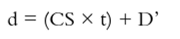
In Figure 6.2 the slope of the regression line describes the athletes CS (m s^-1), whilst the у-intercept describes the athletes D’ (m).

Participants’ CS and D’ from the 3-min test are estimated based on the premise that a runner will expend their D’ within 2.5 min of the all-out effort; consequently, the mean speed of between 2.5 and 3.0 min will stabilise at CS (Burnley et al., 2006). Therefore, D’ from a 3-min running test can be calculated using the following equation (Pettitt et al., 2012), where t = time (sec), S150 s = the average speed for the first 150 seconds of the trial (ms^-1) and CS is the average speed between 150 sec and 180 sec of the trial (m s^-1):

FIGURE 6.2 The linear distance-time model for CS and D based on data from three fixed-distance performance trials

Note: CS = 5.00 m s"¹ and D’ = 100 m.

One potential disadvantage of this assessment method, over the fixed-distance trial approach, is the use of a GPS watch. GPS receiver accuracy is dependent on several factors and may vary between testing days, with Pettitt et al. (2012) reporting the accuracy of measurements during their study at ~3 meters.

An athlete’s CS describes the highest rate of oxidative metabolism, sustainable without a progressively increasing contribution from phosphocreatine and anaerobic glycolysis (Jones et al., 2010). An athlete’s D’ is representative of a fixed amount of work (distance) that can be completed once exercise intensity exceeds CS, and is thought to be predominantly a derivative of anaerobic processes (Jones et al., 2010). Although Jones et al. (2010) explain that D’ is likely to be related to the ‘distance’ between an athlete’s CS and their

vo_2mix.

Normative data for CS and D’ from a cohort of highly trained (mean F0_2max > 70 mL-kg“^l-min“¹) male middle- and long-distance runners were presented by Galbraith et al. (2014a). Data were sub-divided to provide normative data from six 800 m runners, mean CS 4.76 ± 0.22 m-s^-1 and mean D’ 162 ± 44 m, and eight marathon runners, mean CS 5.07 ± 0.31 m-s^-1 and mean D’ 94 ± 49 m. Galbraith et al. (2014b) provided data from well-trained (mean F0_2max> 60 niL kg^-1min^-1) male middle-distance runners, reporting mean CS 4.07 ± 0.28 m s^-1 and mean D’ 106 m. Triska et al. (2017) reported data for a group of recreation- ally trained athletes (mean F0_2max 52.9 ± 3.1 niL-kg ' niitr¹), with mean CS of 3.77 ± 0.35 m.s ¹ and mean D’ 225 ± 72 m. Pettitt et al. (2012) provided normative data for a group of well-trained (mean F0_2max55 ± 4 niL-kg ' niin^-1) female distance runners, reporting mean CS at 4.46 ± 0.41 m.s^-1 and D’ 85.8 ± 40.5 m.

An athlete’s CS and D’ from the field test can be compared to normative data, such as those presented earlier. This can provide an indication of strengths or weakness, which may then inform future training program design. During repeat assessments, an athlete’s CS and D’ can be compared to previous scores from the same athlete providing a useful method to monitor the effectiveness of training programmes and assess whether any adaptations to CS and D’ are occurring.

Research investigating the degree of change in CS and D’ following a period of endurance training are sparse in the scientific literature. Galbraith et al. (2014a) reported small (~2%), but statistically significant, changes in CS during a 1-year training period, in a group of highly- trained (mean V0_2max > 70 mL-kg^-l-min^-1) male middle- and long-distance runners. CS was lowest during August, reaching a peak in February. The increase in CS appears a small change, although it is important to note that the athletes involved in the study were already highly trained with on average an 8+-year training history prior to the study. In contrast, untrained participants have achieved far larger increases in critical power (10-31%) following a 6- to 8-week period of continuous and/or interval cycle training (Gaesser and Wilson, 1988; Jenkins and Quigley, 1992; Poole et al., 1990). D’ showed no statistically significant change throughout a 1-year training period, despite changes of ~24% from August, where D’ was at its highest, to November, where D’ was at its lowest (Galbraith et al., 2014a). In untrained participants, far greater changes have been reported, with Jenkins and Quigley (1993) demonstrating a significant increase in W’ (equivalent to D’) of ~49%, following an 8-week cycle training programme.

To improve CS, continuous or interval endurance training appear important (Gaesser and Wilson, 1988; Jenkins and Quigley, 1992; Poole et al., 1990; Vanhatalo et al., 2008), with total distance covered in training and the volume of time spent at intensities greater than LT velocity shown to encourage an increase in CS (Galbraith et al., 2014a). To improve D’, a training programme focused on power or sprint training appears important (Jenkins and Quigley, 1993). Due to the ecologically valid testing protocols used in the measurement of CS and D’, it has been suggested that the measurement of changes in the distance-time relationship after a training intervention are likely to be of more practical value than the measurements of traditional physiological parameters such as PQ_2nMX and LT (Jones et al., 2010).

Application of Test Data

Aside from the assessment of physical fitness, the CS and D’ values from the test protocols described in this chapter have a variety of potential applications for athletes, coaches and sport scientists. These include prediction of performance, informing racing strategy and the prescription of exercise training.

Prediction of performance: given the previously presented equation, describing the distancetime relationship and it’s individual parameters: d = (CS x t) + D’

Jones et al. (2010) explained that the time-to-exhaustion (t) at a specific constant severe- intensity speed (S), that is any speed above CS, may be estimated using: t = D’/(S — CS). Whilst a further re-working of the same equation will allow the estimation of exercise performance capacity (the quickest time an athlete would take to cover a given distance):

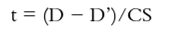
For example, the estimation of time to exhaustion for a runner with a CS is 5.0 m.s^-1 and a D’ of 100 m estimates an endurance time at a velocity of 5.1 m.s^-1 would be 1000 sec, or 16:40 min:sec (100/(5.1 - 5.0) = 1000), and the endurance time at a velocity of 5.3 m.s ¹ would be 333 sec (5:33 min:sec). This information would be useful for a coach aiming to prescribe a challenging but achievable training session (Jones et al., 2010). For the same runner, the estimated quickest performance time over a 3000 m distance would be 580 sec, 9:40 min:sec

((3000 — 100)/5.0 = 580), whilst over 5000 m would be 980 sec (16:20 min:sec). This information may be useful when considering race pacing strategies. Furthermore, this modelling of performance enables the impact of training-induced changes in CS to be quantified. For example, a 2% improvement in CS for this athlete (a change from 5.0 to 5.1 m.s^-1), following a period of training, would correspond to a 19-sec improvement in estimated 5000 m performance time, based on a stable D’ of 100 m. Finally, the modelling of estimated performance time from CS and D’ may be useful in helping athletes decide where their specialism might lie across the middle and long distances. Jones et al. (2010) explain this concept using two hypothetical female distance runners: athlete A, with a CS of 5.85 m.s^-1 and a D’ of 75 m, and athlete B, with a CS of 5.82 m.s^-1 and a D’ of 95 m. Jones et al. (2010) explain that in a competitive race over 1500 m, it can be calculated (using the exercise performance capacity equation) that athlete В would be fastest of the two athletes. However, at 3000 m, the estimated difference between athletes becomes negligible, and for the 5000 m distance, athlete A would have the advantage (Jones et al., 2010).

Informing racing strategy: data on an athlete’s CS and D’ may also prove useful when it comes to determining optimal racing strategy (Jones et al., 2010). The distance-time relationship dictates that optimal performance over a given distance (in the severe intensity domain; covering the middle and the shorter long-distance events) can never be achieved if any part of the race is run at a speed below CS (Fukuba and Whipp, 1999) (see the earlier equations on the prediction of performance using CS and D’). Jones et al. (2010) explain that an athlete may use this knowledge to their advantage in a race, by planning race tactics to suit the relative strengths of their CS and D’ respectively. For example, a race tactic for an athlete with a high CS and a low D’ compared to that of their competitors might be to adopt a front-running strategy, by running at the highest possible speed they can during the race (as dictated by their individual distance-time relationship; see the previous equations for predicting performance). This speed is likely to be above the CS of their competitors, which would require the competitors to run above their CS to maintain pace with the athlete. This would gradually deplete the competitors’ D’, removing their competitive advantage in a sprint finish. Equally, an athlete with a low CS and a high D’ relative to their competitors may be better advised to attempt to slow the race to a pace below their competitors’ CS and then use their higher D’ towards the later stages of the race in a sprint finish (Jones et al., 2010).

Prescription of exercise training: interval training is a popular mode of conditioning in many sports and involves intermittent periods of work and relative recovery (Morton and Billat, 2004). Interval training has the advantage of enabling a greater amount of high-intensity work to be conducted in a single session than would be possible with continuous training (Margaria et al., 1969). Therefore, designing interval training sessions that are individualised to athletes’ specific needs is important. For aerobic training, parameters such as V0_2max, v-V0_2max and LT have all been used to prescribe individualised training intensities (Berthoin et al., 2006). However, Ferguson et al. (2010) explain that an additional consideration when defining exercise intensity is that CS does not occur at a fixed percentage of T0_2lmx. Furthermore, between- subject differences in anaerobic capacity result in the D’ not representing the same volume of supra-CS exercise in all individuals. The consequence of this is that the exercise intensity experienced during an interval training session will be variable between participants unless CS and D’ are accounted for (Ferguson et al., 2010). It has been suggested that an athlete’s CS and D’ can be used to design interval training; setting interval intensity at a percentage of CS and the number of interval repetitions in accordance with the depletion ofD’, thereby inducing the desired training load through the interplay between CS, D’and time to exhaustion (TTE). Morton and Billat (2004) describe this principle based on a linear model, explaining that the depletion of D’ during work (w) intervals and the restoration of D’ during recovery (r) intervals can be estimated as follows: where S = speed and t = time in seconds.

Galbraith et al. (2015) applied this modelling technique to investigate its use in designing track-based interval training sessions for middle- and long-distance runners. Three interval training sessions were designed, with CS and D’ subsequently used to model the estimated point (number of repetitions) at which an athlete would fatigue. Although actual and predicted points of exhaustion were not significantly different, a high typical error was observed for all predicted exhaustion times (Galbraith et al., 2015). Whilst its simple design is appealing, the linear model could not closely predict exhaustion during intermittent running and may therefore not be suitable for the accurate prescription of interval training for middle- and long-distance runners.

Assessment Techniques (ASR)

Bundle et al. (2003) first introduced the term ‘ASR’ into the scientific literature, although in their work the protocol is conducted in a laboratory using a treadmill. The assessment protocol involved the measurement of both anaerobic and aerobic power. The maximum speed supported by anaerobic power was estimated from the highest speed that an athlete was able to maintain for eight steps without a backward drift on the treadmill. This was determined from a series of short high-speed runs at gradually increasing speeds, until the athlete could no longer match the speed of the belt for eight steps (Bundle et al., 2003). The maximum speed supported by aerobic power was determined from a treadmill v-KQ_2mix test (see the previously described v-F0_2max protocol).

A number of field-based assessment techniques have since been proposed for the assessment of ASR, including the recent work of Sandford et al. (2019a, 2019d). In their work, Sandford et al. (2019a) calculated ASR from maximal sprint speed (MSS) and predicted maximal aerobic speed (MAS) performed on an outdoor 400 m athletics track. MSS is assessed via a standing-start 50 m sprint, with athletes performing three maximal efforts with ~3 minutes rest between trials and MSS determined using a sports radar device. On a separate day, a 1500 m time trial was performed for the assessment of MAS (a recent 1500 m race performance time, would be a suitable alternative to a time-trial here).

Interpretation of Test Results and Normative Data

The anaerobic speed reserve can be defined as the speed range an athlete possesses between velocity at v-F0_2max in the laboratory (or maximal aerobic speed in the field) and maximal sprint speed.

When following the treadmill protocol described by Bundle et al. (2003), ASR is defined as the difference between a runner’s maximum anaerobic speed and maximum aerobic speed.

When using the field-based protocol, MAS can be estimated using the following equation (Sandford et al., 2019d):

where 1500v is the athlete’s average speed over the 1500 m trial (km-h ').

The ASR can subsequently be calculated as the ditference between MSS and MAS.

An athlete’s ASR from the field test can be compared to normative data, such as those presented next. This can provide an indication of strength or weakness, which may then inform future training program design. During repeat assessments, an athlete’s ASR can be compared to previous scores from the same athlete, providing a useful method to monitor the effectiveness of training programmes and assess whether any adaptations to ASR (and its components, MSS and MAS) are occurring.

Bundle et al. (2003) report normative data from a small sample of seven trained collegiate athletes (mean F0_2max 61.7 ± 2.0 mL-kg '-min •; range, 53.4-68.0 mL-kg^-,-min^-1). The mean maximum speed supported by anaerobic power was 31.32 ± 1.44 km-h ¹ (range, 27.72- 37.44 km-h^-1). The mean maximum speed supported by aerobic power was 19.08±0.36 km-h ¹ (range, 17.64-20.52 km-h^-1). The mean ASR was 12.24 ± 2.16 km-h ¹ (range, 8.28- 20.16 km-h^-1).

Sandford et al. (2019a) report normative data for MSS, MAS and ASR for a group of 19 international standard (800 m PB of < 1:47.50 min:sec, and/or a 1500 m PB of < 3:40 min:sec) male 800 and 1500 m specialists. Mean (± SD) MSS was 33.55 ± 0.64 km-h^-1; mean MAS was 22.79 ± 0.39 km-h^-1 and mean ASR was 12.24 ± 0.79 km-h^-1, Sandford et al. (2019a) also partitioned their participants into sub-groups of middle-distance runners, reporting mean data for ‘speed types’ (400-800 m specialists), ’800 m specialists’, and ‘endurance types’ (800-1500 m specialists). The MSS of400-800 m specialists (35.48 ± 0.30 km-h^-1) was faster than the 800 m specialists (33.68 ± 0.63 km-h^-1), and 800-1500 m specialists (31.49 ± 0.99 km-h^-1). MAS in 400-800 m specialists (22.41 ± 0.62 km-h^-1) was slower than both 800 m specialists (22.76 ± 0.50 km-h^-1) and 800-1500 m specialists (23.21 ± 0.06 km-h^-1). ASR of400-800 m specialists (14.46 ± 1.00 km-h^-1) was larger than 800 m specialists (12.12 ± 0.61 km-h^-1) and 800-1500 m specialists (10.13 ± 0.76 km-h^-1).

Application of Test Data

The importance of a high ASR to a middle-distance runner can be substantiated by the work of Bundle et al. (2003) and Sandford et al. (2019a, 2019d). Bundle et al. (2003) report that the ASR protocol allows high-speed running performance to be accurately predicted from an athlete’s maximum anaerobic and aerobic power. This highlights ASR as an important determinant of performance particularly in middle distance events over 800-1500 m. Sandford et al. (2019a) report that MSS and ASR displayed strong negative (r = -0.74) relationships with 800 m performance time. For the international-level athletes tested, a faster MSS (and therefore ASR) is likely to be strongly related to a faster 800 m performance. Interestingly, for the same MSS, a faster MAS or ASR was not strongly related to changes in 800 m time. Sandford et al. (2019a) suggest therefore, that at an elite level, faster 800 m runners will have a larger ASR (as a consequence of a faster MSS), combined with an already established minimum level of MAS. Therefore, once a certain aerobic standard (MAS) is reached, MSS becomes a differentiating factor in elite 800 m runners (Sandford et al., 2019a).

Summary

To measure the important physiological determinants of distance running performance, and thus evaluate a runner’s relative strengths and weaknesses, a wide range of laboratory and field-based assessment options exist. Differences in physiological testing profiles between athletes can explain differences in distance running performance. Laboratory-based physiological assessment should include maximal oxygen uptake (K0_2nMX), running economy (RE), lactate threshold (LT) and the velocity associated with V0_2max (v-D0_2lmx). Field-based physiological assessment should include critical speed (CS), the maximum distance that can be achieved at speeds above critical speed (D’) and the anaerobic speed reserve (ASR).

7