Method
Unified Feature Representation with Imputation
In this section, we present our method with subspace embedding diagram as shown in Figure 13.4, where source and target datasets are projected in a common latent space and a generic classifier is learned to distinguish the labels. Given source and target datasets 7?s- and ©y with N and M (N&M) samples, to apply CCA in both datasets, the number of instances should be identical, which is not likely for real-world scenarios. We propose a method for pairing, which is finding the nearest pair for the dataset with the smaller number of instances (target) in another one (source) by aligning the feature space first.
Assume we have two datasets with common binary label y, namely, domain source and target source, which are denoted as T>s and Py, respectively. As the two databases are not fully aligned, we split the feature space

Figure 13.4 Subspace embedding learning representation.
into three components according to the missing rate, e.g. common features Fc, target-specific features FT and source-specific features Fs as shown in the Figure 135, where Fc are the features that both and T>t observe, and here, the term ‘observe’ entails that the observed instances are substantial enough for each feature (at least one observation). Fr contains features that are only observed in the target and is totally missing in the source, and similarly, Fs consists of features observed in the source and is totally missing in the target.
More formally, given two datasets, namely, source domain T>$ and target domain regarding the same binary label f G {0,1}. Input feature spaces for each domain are denoted as (Vs and Xt■, and then, we define common feature space Fc = Xs r>Xr, target-specific feature space FT = XTFsw and source-specific feature space Fs = Xs F.-.
The imputation involves two procedures, which are cross-transfer imputation and feature creation imputation. Cross-transfer imputation aims to fill the missing values in Fc using existing imputation techniques, while feature creation imputation can be achieved in two ways: the first is to complete FT for the source set and Fs for the target set by utilizing the data from target and source, respectively, and the second is to simply pad zeros for missing values in Fr and Fs.
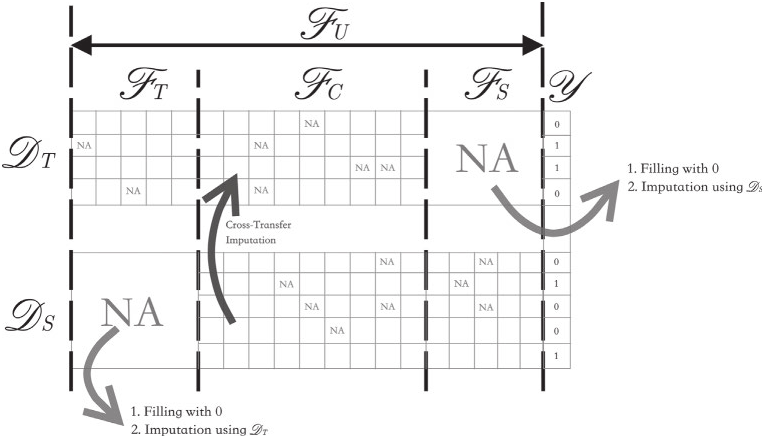
Figure 13.5 Unified feature representation for two datasets T>t and T>s. NAs in grid suggest data are missing, observed feature entries are left blank and two large NA indicate that FT and Fs in T>s and T>s are totally missing. Cross-transfer and feature creation imputation are performed on source- and target-specific features.
Nearest Pairing Methods
For each sample in the target dataset, we desire to identify the most similar one from the source dataset. We propose a heuristic pairing algorithm in this section. First, the distance matrix (NxM) is created using Euclidean metrics. Each column represents source indices between all source instances and one specific target instance sorted by distance in ascending order. That is, the first row represents the target index where target instance and source instance have minimal distance and vice versa. Then, in the first row of the distance matrix, we find the largest number of non-replicated instances from the source and then delete these paired instances from source and target until all pairings are finished. The algorithm is shown below.
Algorithm 1: Nearest Pairing
Input: Source with N instances, target M instances, assume M
Output: Paired source and target datasets.
Step-1: Data normalization and pre-processing;
Step-2: while Instance(P _5 ) > 0 do
{
Dist _Mtx <— Euclidean _ Distance(Ds,Di ,
Find largest non-replicated pairs in the first row, which are denoted as Ps-/>, Py/>;
P$ <— Ds D$ p
Py <— Py Py yg
}
Step-3: Return Ps, Py.
CCA Transformation
Algorithm 2: Classification with Nearest Pairing
Input: Source: Ps g 7?"'Xi/s, target: Py G R"T*‘‘T, assume ns
Step-1: p <— observed_features(Ps );
Step-2: p <— observed_features(Ps);
Step-3: p <— p n p;
Step-4: Data normalization and pre-processing;
Step-5: Cross-transfer imputation with kNNI;
Once we obtain the paired source and target datasets, we can apply the linear CCA with regularization (Equation 13-4), the kernel CCA (Equation 13-6) or the deep CCA (Equation 13-7) for finding a common latent space. A classifier is then employed in the common latent space. Details are shown in Algorithm 2.

