Position and Wave Function

Consider again the two slit experiment shown in Figure 3.1, generalized to an N-slit experiment:

Letting N -> oo, then it is necessary to introduce a continuous label q :

So, the component of say, |*P) in the basis q) is now a function of the continuous variable :

Considering the orthonormalization relation then

or

Relation 3.9 is the probability amplitude for measuring the eigenvalues q of the position operator q . This implies that |^VP(^)|² should be the probability density in q-space. From here

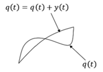
FIGURE 3.1 The classical or true path q( t), the false path q(t) and the quantum fluctuation y(t) around the classical path.

So, the closure relation of the eigenvector |q) (showing the particle must be somewhere) can be written in the following form:

Here, I is a unit matrix. For the probability interpretation to be feasible as seen earlier it is necessary the completeness relation:

Here, the probability that the particle will be detected in the interval between q and q + dq:

So, 4%) is the spatial wave function of wave mechanics and |4^,(^)|² is the relative probability of the particle position located in the interval between q and q + dq.

We rewrite the operator in 2.80 via the continuum position operator form:

Then, considering 7, we have

From equation 3.14, we evaluate the expectation value of q in the state IT*):

Rather than limiting ourselves to the finite interval (a, b) we set a -> - oo and b -* oo so that q e (-00,00). So, the transition amplitude for the continuously-infinite slit experiment can be rewritten:

Momentum Space

From the above developments, we move to momentum space by using the Fourier transform basis:

From here, the following amplitudes are referred to as momentum space wave functions:

I

These are just unnormalized plane waves describing free particles of momentum p with the momentum states p) satisfying the orthogonality relation:

Here, S(p - p') is the Dirac (5-function. The completeness relation:

We construct a Hermitian operator p:

Then

These states will be generalized to eigenstates of Heisenberg representation-operators by selecting

Note that these are eigenstates of the Heisenberg representation q{t), not the result of allowing q, t) to evolve with time, where t„ is an initial time moment.