Stationary Phase Method/Fourier Integral
Further, in chapter 8 we will be studying an important and powerful approximation method known as the Wentzel-Kramer-Brillouin (WKB) method, where interest will be oscillatory integrals of the form:

Here,/(q) and S(q) are assumed smooth functions and independent of ft. The integral of the form in 5.2 mimics the Fourier integral and S(q) the phase or phase function. We examine the asymptotic behaviour of the integral Jp[ft] for small ft, (ft -> 0), i.e., for the quasi-classical approximation. We will not consider the trivial cases when

or

If,

then the integral 5.2 becomes the Fourier transform:

The function

for small ft, (ft —> 0) rapidly oscillates and yields two neighboring half-waves of approximately equal areas but opposite in sign. So, the sum of the areas is an infinitesimal quantity and consequently the following integral is also an infinitesimal quantity according to the Riemann-Lebesgue lemma:

For the finite integral
 then

The rate at which the given integral tends to zero is dependent solely on the properties of the derivatives of the function f(q).
Suppose the functions/^) and S(q) are infinitely differentiable and S{q) Ф 0 for any q belonging to the interval [a,b], then as Pi —> 0 , we investigate on the principal term in the asymptotic expansion ^[ft]
from equation 5.2. Letting A = —, we do integration by parts in 5.2:
ft

Here,
 then from

it follows from Riemann-Lebesgue lemma that
 Letting,

then

and carrying out integration by parts then

Here,
 then from

it follows from Riemann-Lebesgue lemma that

So,

The last term should be the correction to the formula.
Contribution from Non-Degenerate Stationary Points
The above study does not give room for the phase S(q) to have a stationary point within an interval. This implies that

for q defined within the interval [a, b]. If such a stationary point exists then the asymptotic behavior of the integral .F[A] will be of a different nature than that shown above.
Consider the phase

So,

This has a stationary point q = 0 and is depicted in Figure 5.1. At the neighborhood of this stationary point, the function cosXq2 is not oscillatory. So, the sum of the areas of the waves in the cosine is sufficiently less than that at the stationary point. Hence, the value of the integral JF[A] is of order A 2.
If the function/(q) should be infinitely differentiable in the interval [0,л] then

Here, sgna denotes the sign of a.
We show the truthfulness of this equation by letting

then,

or

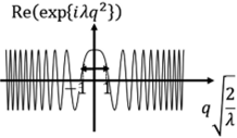
FIGURE 5.1 showing only a small region at the neighborhood of the extremum q = 0 contributes to the integral of equation 5.24 in stationary phase approximation.
Hie first integral yields
 then the second integral yields
 So,

Let,

where, we introduce an infinitely differentiable function/,^) for q belonging to the interval [0, д]:
 So,

We study the last term:
 or

or

So, from 5.34 we have

From here and established by analyses of Figure 5.1, the dominant contribution to the integral comes from a region of size -j=, about the extremal (critical or stationary or saddle) point of the function
S(q). Outside of this region, the integrand is rapidly oscillating and so gives to leading order a negligible contribution.

