Moments of IIMs With Applications

The ПМ H_k| from (1.15) is not an unbiased estimator of the population ПМ, H_ki from (1.13). But, U_ki and X are obviously unbiased for the respective parameters <5и = hi,г = £/ [14/] ^ar>d the population mean // = //f. Theorem 1.2 presents the asymptotic distribution of the estimator H_ki, indicated by Л

TABLE 1.9

Difference 1д-1ц in the Values of the IIMs

for positive integers к, l such that к + 1 = m(< n). Theorem 1.3 provides an expression for the MSE associated with H_kk

Theorem 1.2. If non-negative i.i.d. observations X_k/X2,..., X„ are such that Ер [X⁴] exists, then the asymptotic distribution of H_ki is given by:

where,

Proof: Both U_ki and X are U-statistics with respective degrees m and 1. Their joint limiting distribution would be bivariate normal. Now, U_k) unbiasedly estimates <5_W- Hence, using Hoeffiding (1948), we get, with cr as defined in Theorem 1.2

Next, let us verify that

with Q defined in Theorem 1.2. Using Lee (1990, p. 17), we can express:

where

Using Hoeffiding (1948), we can claim:

The second conclusion is a restatement of the central limit theorem.

Then, we obtain the following asymptotic bivariate normal distribution:

as n —> oo.

Thus, we have the following asymptotic distribution for the ratio of the two U-statistics, namely U_kl and 2X:

with f² defined in Theorem 1.2 the proof is complete. ■

Theorem 1.3. If non-negative i.i.d. observations Xi,..., X„ are such that we have Ef[X^4+e]finitefor some e> 0, then the asymptotic MSE of the estimator H_kt is given

by-

assuming 0 < £² < oo with f² = fp defined in (4.1)

Proof: Using Hoeffding's (1948) decomposition, we have:

where gj's are themselves U-statistics of degree j based on the kernel

Uj(Xn,... ,Xjj) with

where Л, = Ei<,_C,x_ic)

Using Lee (1990, p.30), we have Ef[g? ] = 0(n~²). Next we can write

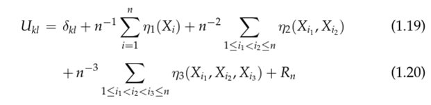
with R„ = op(n~³/²) and also:

Next, using Hoeffding's (1948) decomposition of the sample mean, we obviously have:

We also note that and

Under the assumption that Ef[X⁴⁺⁶] < oo, we observe that

Thus, the required conditions (1.1)-(1.7) and (1.4)-(1.6) from Maesono (2005) are clearly satisfied. Now using the variance and covariance formulas for U- statistics (Lee, 1990), we have:

Hence, applying Theorem 2 of Maesono (2005), we immediately obtain an expression for the asymptotic MSE (AMSE) of H_ki as follows:

Hence the theorem is proved. ■

A Consistent Estimator of ξ Defined Via (4.1)

We observe that H_k] is a strongly consistent estimator of в_к! since (J_w and X are both strongly consistent estimators of S_kt and ц respectively. Now, let us obtain a consistent estimator for the parameter defined via (4.1).

First, we go back to the expression of £ from (4.1). Upon generalizing Xu (2007), we have an estimator of £ as follows:

where we define:

We note that £„ from (1.21) is an unbiased estimator of £ and it is a U-statistic involving a symmetric kernel of degree m. It is well-known (Hoeffiding,

1961) that any U-statistic is a strongly consistent estimator of its expectation under an appropriate moment condition. Hence, the estimators £„ as well as the sample variance S² are strongly consistent estimators of ( and a² respectively.

Next, it remains to find a strongly consistent estimator of a. Along the lines of Sen (1960), Sproule (1969), and Sen and Ghosh (1981), for each j = 1,..., n, let us define a U-statistic:

where fly = {(h, i₂,..., i_m) :l 2< ... < i_m < n and i, i₂,..., i_m Ф/}■ See also Sen 1999,2005.