Simulation Study

We note that under the distribution-free scenario, the purely sequential procedure for estimating population mean developed in Ghosh and Mukhopad- hyay (1979) used sample SD as an estimator of the population SD. We define the stopping rule based on the sample SD as developed in Ghosh and Mukhopadhyay (1979) as

and we denote Rn_sd (//.) as the expected cost of estimating the population mean /x using the sample mean based on Nsd observations.

We now demonstrate and compare the properties of the proposed purely sequential procedure based on GMD (N) with the purely sequential procedure developed in Ghosh et al. (1997) using a Monte Carlo simulation study. Kindly note that in order to differentiate between the final sample size for SD-based procedure (Nsd) from that for GMD-based procedure, we rename N, which was defined in (5.7), as Ngmd-

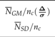
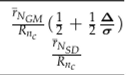
We considered several underlying distributions of the data, namely: normal (N(mean, variance)), gamma (Gam(shape, rate)), lognormal (LN(location, scale)), Pareto (Par (scale, shape)), and mixture normal (pN (mean, variance) + (1 - p)N(mean, variance),p € (0,1)). To implement the purely sequential procedure, we proceed as described in Section 5.2. The number of replications is 5,000. In Table 5.1, we report the mean sample size based on GMD (Nqm) with its standard error (s(Ngm)), the mean sample size based on sample SD (Nsd) with its standard error (s(Nsd)), the mean expected cost (r^_CM) and its standard error (s(f/v_CM)), and the mean expected cost (r^_sl}) and its standard error (s(r^_SD)) based on 5,000 replications via Monte Carlo simulations by drawing random samples from the above-mentioned distributions.

TABLE 5.1

Estimated Average Final Sample Size and Sample Mean

Distribution
N(30,102)	113.0488 (0.1096)	100	1.1305 (1.1284)	2001.8180 (2.0520)	1.0009 (1.0642)
A = 81000, c = $10	99.9384 (0.1036)		0.9994	1984.3200 (2.0718)	0.9922
N(200,202)	356.8250 (0.1937)	317	1.1256 (1.1284)	1271.2180 (0.7121)	1.0025 (1.0642)
A = $500, c = $2	316.0568 (0.1791)		0.9970	1261.4660 (0.7159)	0.9948
G«»;(10.78,0.84)	43.7758 (0.0747)	40	1.0944 (1.1154)	4289.9458 (7.4837)	1.0725 (1.0577)
A = $5000, c = $50	38.9150 (0.0735)		0.9729	3802.3042 (7.3769)	0.9506
G«»i(2.6,0.4)	137.2818 (0.1518)	128	1.0725 (1.0757)	2727.7897 (3.0389)	1.0655 (1.0379)
A = $10000, c = $10	126.8840 (0.1673)		0.9913	2520.1624 (3.3496)	0.9844
LN(2.51,0.562)	88.5230 (0.1510)	88	1.0059 (1.0138)	8774.0473 (15.0996)	0.9971 (1.0069)
A = $5000, c = $50	85.1314 (0.1903)		0.9674	8436.5043 (19.0298)	0.9587
£,N(2.51,0.562)	281.2396 (0.2697)	278	1.0117 (1.0138)	5608.9348 (5.3929)	1.0088 (1.0069)
A = $10000, c = $10	275.1020 (0.3631)		0.9896	5486.6923 (7.2635)	0.9868
P«r(1000,10)	1044.4362 (0.6220)	1112	0.9393 (0.9415)	52186.0169 (31.0986)	0.9386 (0.9708)
A = $2000, c = $25	1104.8278 (0.9278)		0.9936	55207.9438 (46.3860)	0.9929
P«r(3000,8)	4570.4778 (1.3774)	4949	0.9235 (0.9238)	456977.4553 (137.7348)	0.9234 (0.9619)
A = $5000, c = $50	4943.1432 (2.2859)		0.9988	494248.6514 (228.5892)	0.9987
0.5N(30,52) +0.5N(60,102)	60.8280 (0.0838)	54	1.1264 (1.1350)	12037.18 (16.8092)	1.1146 (1.0675)
A = $1000, c = $100	53.3452 (0.0864)		0.9879	10541.47 (17.3392)	0.9761
0.2N(50,102) +0.8N(100,102)	149.5622 (0.1567)	142	1.0533 (1.0587)	14881.80 (15.6822)	1.0480 (1.0293)
A = $2000, c = $50	141.2000 (0.1270)		0.9944	14050.48 (12.7114)	0.9895

The optimal sample size (n_c), the ratio of average final sample size to the optimal sample size (Ngm/пс), and the ratio of the expected cost for a sample of size Ncm to the average cost for a sample of size n_c(^rdj^-) are also reported.

From Table 5.1, it can be observed that on the average, the GMD-based procedure gives a final sample size that is mostly more than that of the SD-based procedure except in one case for the lognormal distribution. However, neither of these two procedures has a clear upper hand when it comes to the standard error of the estimate of the optimal sample size; the GMD-based procedure has a lower standard error for the estimate of sample under the lognormal and Pareto distributions while the SD-based procedure has a lower standard error under the normal distribution (see second column). The fourth column shows that on an average the ratio of the final sample size for GMD-based procured to the optimal sample size, is close to A/a as stated in Theorem 5.1. In the fifth column of the table, it can be observed that the GMD-based procedure provides estimates for the risk with lower standard errors as compared to that of the SD-based procedure. The GMD-based procedure performed well in terms of lower risk function in the case of the Pareto distribution than in the case of the SD-based procedure. This supports the claim that GMD-based algorithms are more robust. The last column suggests that the ratio of the cost of estimating the population mean using the final sample size, given by the purely sequential procedure to the minimized expected cost is close to (0.5 + 0.5Д/(т) for GMD-based procedure and 1 for SD-based procedure. Thus, our purely sequential procedure works remarkably well in these three distributions as well.