The Proposed DC-DNN Model

The process involved in a cloud-based image retrieval system is shown in Fig. 9.1. The training images and testing images undergo the DC-DNN process in the cloud server to retrieve the related images. The complete operation involved in the DC-DNN technique has illustrated in Fig. 9.2. From the figure, it is clear that the DLTerQEPs and Crest lines models are used as a feature extractor to derive the texture and edge features. Then, the affinity among images placed in a database and QI has been computed in the feature space with the help of the Euclidean distance value. After the images are retrieved, DNN-relied image classification is carried out.

DLTerQEP-Based Texture Feature Extraction

DLTerQEP explains the spatial local texture in the case of ternary patterns under the application of local extrema and dimensional geometric infrastructures. For

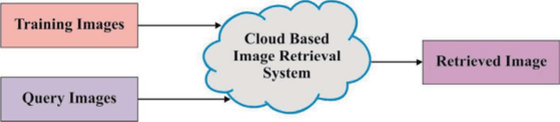
FIGURE 9.1 Cloud-based image retrieval system.

FIGURE 9.2 Overall process of proposed DC-DNN model.

DLTerQEP, local extrema in each direction are essential to computing with local differences from middle and adjacent pixels by indexing the patterns with pixel locations.

The locations undergo indexing using four directional extremum operator evaluations. Local directional extrema values (LDEV) for local pattern neighborhoods of an image (IM) are valued in Eq. (9.1)

where the size of input image is Zi x Z. The four directional, HVDA-i structures of possible dimensional local quinary patterns (LQP) geometries is used in the feature extraction operation. The directional local extrema in 0°, 45°, 90°, and 135° directions have been extracted in HVDA7. Following, four Directional Ternary Extrema Codings (DTECs) are collected according to additional four directions from different thresholds under the application of the local ternary patterns (LTP) model.

Crest Line–Based Shape Feature Extraction

Here, it is developed with automated crest line extraction of used medical images. It is comprised of three phases. Initially, a step that has initial curvatures and directions on all vertices of triangulation, the next step manages crest point classification, and the last step is to monitor the crest lines.

Curvature Approximation

The initial step is:

For each vertex V; of a mesh,

• 1. Obtain the star of v,, pointed by a star(vi).
• 2. Fix the quadratic patch (2) on v, and star(vi).
• 3. Determine the principal curvatures as well as the adjacent directions on v,, as defined in the previous stage.

Crest Point Classification

In crest line, a vertex point has been identified as the crest point. The local neighborhood of vertex v of the triangulated mesh is a star(v). It is applied as well as directly evaluates the directional derivative of the maximum curvature of all vertices, but the gradient is noise sensitive and does not offer the reliable measures when required, especially on irregular triangulated meshes. Finally, the given rules were applied in this method. Once the higher principal curvature k and corresponding domain direction t, on vertex v are calculated, some of the domain values of the star(v) are given in the following:

• • The domain measures of star(v) are (U|U,.), where L represents a value of vertices in star(v) and u_u denotes the domain of v.
• • Identify the facet that conjunction t and obtain two vertices u,„; and u,„₂, m{ 1, 2} ell. L.
• • Follow a similar direction-?; and obtain vertices u_;1 and u,₂, j {1, 2}e [1, L.
• • Obtain maximum curvatures k™¹"'² ,k{'¹² on points U„,;_m2 and U_ylj2 by interpolating with (k"' k"’²) and (kj',k{²).
• • If (k[)² - (£|'"^lm2)² >e and (fc,⁰)² ~(k{'^j2)² >e then v is a crest point, where e > 0 manages the maximally.

It has been employed to limit the arithmetic errors on the number of crest points. In addition, k{ implies the largest curvature on vertex u,,0

Crest Lines

The model is comprised of managing sources in crest point classification. However, it has been reached to find the crest vertices that are not applicable. Also, there is a requirement of developing technology to combine all points and deploy features of an object. It is constrained with two portions. Initially, it is observed with every crest line and, secondly, it concatenates the massive number of lines, respectively.

Suppose the mesh is comprised of N vertices. The steps are:

• 1. Initiate line list LS and fix several lines j = 0.
• 2. Fix the id of recent vertex i = 0.
• 3. When v, is not visited, if a crest point contains two crest points on the star then:
  • • call traceCrestLine(yi, lsj,(Vj, Isj, “first”).
  • • call traceCrestLine(yi, ls_h (v,, Is,, “last").
  • • Improve j.
• 4. When i < N. increase i and go to Step 3.

When a crest point is constrained with one or more crest points on the star and classified into a cross crest point, the start tracing line leads to the issue of the ambiguity of choosing a path. A cross crest point is named as a bifurcation point. A crest line bifurcates more than two lines. Due to the lack of advance link of a point, until tracing stop criteria and apply the latter portion of join lines.

The procedure traceCrestLine (vt, Is,) is:

• 1. Mark v, as visited and include it to line Is,.
• 2. Obtain every vertex of star(vi), which are crest points that are not visited. Suppose their number be n.
• 3. When n = 1, then go to Step 1 for novel vertex, otherwise exit.

Euclidean Distance–Based Similarity

In the content based medical image retrieval (CBMIR) method. Euclidean distance has been used for identifying similarity from the images. The distance from two images is employed to compute the similarity between images. Euclidean distance is one of the vital distance values. It is computed with the application of the Minkowski Distance equation by fixing p’s value as 2. For tw'o diverse images .v and y, it upgrades the distance d using the equation

DNN-Based Classification

The DNN basically operates on the feed-forward networks model along with the greedy layer. In this model, the data flow is initiated from the input layer to the output layer with no looping task. A major benefit of the DNN classification model is the probability of a missing value is minimum. The DNN concept implements with a single layer in the unsupervised pretraining phase. The DNN model determines a classification value f(x) at the prediction time. Each input data т = [x,.....лгд,] is named as forward pass. Here, / implies function that has a series of layers that is shown in Eq. (9.3)

where input layer is denoted as x,, output layer is x, are model parameters; and g(Z,) analyzes the mapping task. Layer-wise relevance propagation degrades the classification as output/(л^-) with respect to relevance’s r_r which has input component x,, which involves in the classifier decision as given in Eq. (9.4)

where r, > 0 is the positive classification decision and r, < 0 is negative evidence; otherwise, it is referred to as neutral evidence, although the relevance attribute r, is computed under the application Eq. (9.5). The common structure of a DNN is presented in Fig. 9.3.

The DNN is capable of examining the unknown feature coherences of input. The DNN offers a hierarchical feature learning method. Hence, the higher-level features can be retrieved from minimum level features with a greedy layer-based unsupervised pretraining stage. Hence, the main goal of a DNN is to manage the complex functions that present high-level abstraction.

FIGURE 9.3 DNN architecture.

TABLE 9.1

Data Set Description

Description	Values
Database	NEMA CT
Number of Images	600
Image Size	512x512
Number of Classes	10
Classes Distribution	54. 70. 66. 50. 15. 60. 52, 104.60.69