Frequency Distribution
A frequency distribution is one of the simplest ways to represent a single variable. It provides a comprehensive overview of a dataset at one glance. For a categorical variable (e.g., seasons) or a small number of numeric cases (e.g., number of cars per household), each possible value may represent a group in a frequency table. When the set of data values are spread out (e.g., housing price), however, it is difficult to set up a frequency table for every possible value. In this case, class intervals are used to group the data. For class intervals, after identifying the maximum and minimum values of a variable, the entire dataset is broken down into a number of subintervals of equal length that covers the range between maximum and minimum values without overlapping. By simply counting the number of observations in each subinterval, we get the ‘frequency’ of each cell or group. A table of frequencies is drawn up by counting the observations in each group.
For ease of understanding, relative frequency may be calculated for each group. Relative frequency for each group is the fraction of observations belonging to that class.
Relative frequency of a group is:

The frequencies can be represented either in a table format or by a relative frequency histogram. A histogram is simply a way of representing the relative frequencies visually (see Figure 7.4 for an example). The class intervals are marked on the horizontal axis of the graph, and for each interval a vertical bar (rectangle) is drawn whose area is equal to the relative frequency of that interval.
Central Tendency
In statistics, a measure of central tendency is an estimate of the center of a distribution of values. This central value can be measured as a mean, median, or mode.
The most commonly used measure is the mean of a dataset, which is the total of all the observed values divided by the number of observations. The formula for the mean is as follows:
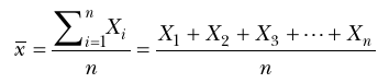
where
S = Summation of all values
X= Refers to individual numerical values
n = Total number of observations
i = A counter, which identifies the first xwhen i = 1, the second xwhen i = 2, and so on to the last, or the nth, when i = n
The mean is the only measure of central tendency that can be used in inferential statistics to infer characteristics of a population from which the sample is drawn. The mean can be computed only from interval or ratio scale data. However, the major drawback is that one single observation that is vastly different from the rest of the observations can seriously skew the mean of the entire dataset, giving a faulty estimate of the same. These extreme values are referred to as outliers.
The median of a dataset is the middle value of the observations when they are ordered from lowest to highest in value. When the number of observations is odd, the median is the middle number of the total number of observations. In other words, median is that value of a dataset that divides the dataset in two equal halves. Where there is an even number of observations, the median is considered to be the number halfway between the two middle observations (i.e., mean of the two numbers).
For any given set of data, the median is less sensitive than the mean to extremely low or high values, so it is often used to protect against undue influence by outliers. For a skewed distribution, such as with income, the median is more typical of the sample than is the mean. Due to outlying values of income (the 1 percent of super-rich individuals), the mean of income will be higher than what is typical for those in the sample.
If the number of samples is quite large, then it is sometimes useful to extend the concept of median and divide the dataset into four equal parts rather than two. Each part is then a quartile. Or samples can be divided into quintiles (five equal parts) or deciles (ten equal parts).
The mode of a dataset is the most frequently occurring observation within the data. The advantage of using mode is that it can be computed with nominal or ordinal data, as well as interval and ratio scale data. While a mode is a good way to tell the most common attribute, there are shortcomings. First, if no value occurs more than once, there can be no mode. Second, if multiple values occur more than once, there can be two or more modes.
Which is the best estimate measure of central tendency to use in planning: the mean, the median, or the mode? The answer is not simple because the choice depends on the purpose. The mode has the disadvantage that it is not influenced at all by the distribution of scores at values other than the mode. The median takes into account more data than does the mode, in that it requires the number of scores to either side of the median to be equal. Yet, the median is not influenced by the size of the scores. In contrast, the mean takes into account every' score in the distribution; however, there are cases where using the mean can be misleading (e.g., presence of outliers). One has to cautiously choose a measure of central tendency that describes the data most accurately, noting that sometimes this includes using more than one type of measure.
Dispersion
In addition to locating the center of the data, an important aspect of a descriptive analysis is to numerically measure the extent of variation around the center. Two datasets may exhibit similar positions of the center but may be different with respect to variability. Thus, datasets should also be analyzed for dispersion around the mean. There are three common measures of dispersion: the variance, standard deviation, and range.
A small variance indicates that data points tend to be very close to the mean, while a large variance indicates that data points may be very spread out from the mean and from each other. Some of the deviations from the mean—differences between the observed values and the mean—will have positive values (be above the mean), and some will have negative values (be below the mean). If we simply summed them, the negative values would cancel the positive values. So for the purpose of computing a measure of dispersion, we square the deviations from the mean to get rid of the negative signs. The variance of a set of data is denoted by s2 and is defined as the sum of the squared deviations from the mean divided by the number of observations minus one. The formula for the variance is:
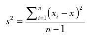
where
S = Summation of all values
n = Total number of observations
i = A counter, which identifies the first »when i = 1, the second x when i = 2, and so on to the last, or the nth, when i = n
x = Mean value of observations
For a sample, subtracting one in the denominator gives us an unbiased estimate of the sample variance. For a population rather than a sample, the formula remains the same except the denominator becomes n, rather than n — 1.
The variance is one power above, i.e., a s^warcvalue, the unit of the dataset. To have the measure of variation and the observations in the same units, the square root of the variance is more commonly used. This is called the standard deviation of a set of values.
The standard deviation of a set of n observations is denoted by s. The formula for the standard deviation of a sample is:
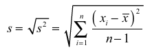
where
S = Summation of all values
n = Total number of observations
i = A counter, which identifies the first x when i = 1, the second x when i = 2, and so on to the last, or the nth, when i = n
x = Mean value of observations
Again, a low standard deviation shows that data observations tend to be very close to the mean, whereas a high standard deviation indicates that the data observations are spread out around the mean.
Range is the difference between the highest and the lowest value of a dataset. It does not provide much detail about the nature and characteristics of the dataset. For interval and ratio scale data, the range is the difference between the two extreme values.
but for ordinal data it is the number of categories used to describe the data. There are few statistical procedures based on the range. It is mostly used as a quick substitute for, or used as an addition to the standard deviation, as a measure of the width of the distribution. It is seldom reported in planning articles.

