Mechanics
Pearson Correlation Coefficient
The mathematical formula for computing the Pearson correlation coefficient ris:
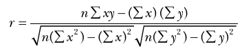
where n is the number of pairs of data and x and y are the two variables.
We present a second equivalent formula that is harder to compute but easier to interpret.
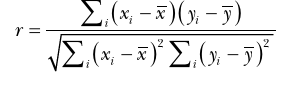
where x and y are the means of x and y.
Positive correlation: If xand y have a strong positive linear correlation, rwill be close to +1. An rvalue of exactly +1 indicates a perfect positive fit (all points lying on an upward sloping line).
Negative correlation: If x and y have a strong negative linear correlation, r will be close to -1. An rvalue of exactly -1 indicates a perfect negative fit (all points lying on a downward sloping line).
No correlation: If there is no linear correlation or a weak linear correlation, rwill be close to 0. A value near 0 means that there is a random (or conceivably a nonlinear) relationship between the two variables.
A key mathematical property' of the Pearson correlation coefficient is that the value is invariant to changes of location and scale. For instance, when the variable x is linearly transformed to a + bx, where a and b are constants, the correlation coefficient with y does not change. This makes sense. If the relationship between two variables exists, the correlation coefficient will pick up the relationship regardless of how the variables are measured.
The Pearson correlation coefficient is only' appropriate for examining the relationship between continuous variables (interval and ratio scale variables such as VMT and fuel price), not nominal or ordinal measurements. In addition, both variables should be approximately normally distributed (i.e., a bell-shaped curve in a histogram). Also, the Pearson correlation coefficient only measures linear relationships (Lee Rodgers & Nicewander, 1988). It is possible that while ris close to 0, there is strong nonlinear relationship between the variables (see the third row in Figure 9.1).
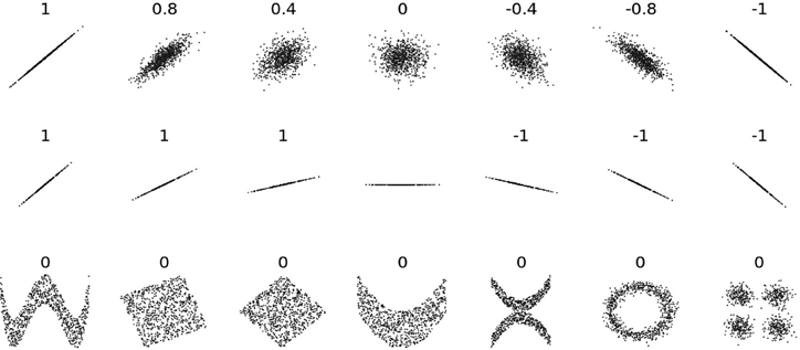
Figure 9.1 Scatterplots and Pearson Correlation Coefficients
Source: https://cominons.wikimcdia.Org/wiki/File:Corrclation_exaniples2.svg
Spearman Correlation Coefficient
In statistics, a rank correlation coefficient measures the degree of similarity between two rankings, and can be used to assess the significance of the relation between them. Continuous variables (interval and ratio scale variables) can be ranked and analyzed this way. Ordinal variables can also be ranked, and hence the relationship can be analyzed this way. For example, urbanized areas can be ranked in terms of VMT per capita and fuel price, and the rankings can be compared. Or cities might be (and often are) ranked in terms of livability and economic performance, and the rankings can be compared.
The Spearman correlation coefficient has a wide range of applications because there is no strict requirement of data condition—neither linear relationship or normal distribution (Philips et al., 2009). Regardless of the distribution and the size of sample, the Spearman correlation can be used as long as the two observations are paired.
The rank correlation statistics are as follows:
- • Spearman’s correlation coefficient
- • Kendall tan correlation coefficient
- • Goodman and Kruskal’s gamma coefficient
Of the three, the most popular correlation statistic is the Spearman’s correlation coefficient (rj.
The Spearman correlation coefficient is just the Pearson correlation coefficient for data that is rank ordered (Myers, Well, & Lorch, 2010). Two variables x and y are converted to the rankings x and y, and then the formula for the Pearson correlation is applied to them.
Naturally, since the same formula is applied, the Spearman correlation coefficient is like the Pearson correlation in that it falls between +1 and -1. Like in the Pearson correlation, the sign of the Spearman correlation coefficient indicates the direction
154 Guang Tian, Anusha Musun uru, and Reid Ewing
of the association between x and y. If y tends to increase with x’s increase, rs is positive. Or, if y tends to decrease with x’s increase, rs is negative. When r( equals 0, there is no tendency for y to either increase or decrease when x increases.
Intraclass Correlation Coefficient
In statistics, the intraclass correlation coefficient (ICC) is used to measure the correlation of variables representing different measurements of the same phenomena. The ICC is most often used to test the reliability or equivalency of measurements, one rater versus another, one variable versus another (see Chapter 6).
The Pearson correlation coefficient r between rater 1 and rater 2 can be represented as:
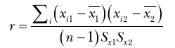
Conversely, the ICC is:
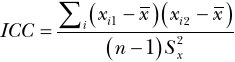
where x is the mean, x, and x2 represent two raters, and ,Sj is the standard deviation.
The key difference between ICC and ris, then, the estimation of mean and variance. For the Pearson correlation coefficient, the mean and variance are calculated separately for the two groups. But for ICC, they are the aggregate of the two groups.
The ICC is the preferred measure of inter-rater reliability when cases are rated in terms of some interval variable or interval-like variable, such as a Likert scale measurement (Alexander, Bergman, Hagstromer, & Sjostrom, 2006; Ewing et al., 2006). The Pearson correlation coefficient is sensitive only to random error (chance factors), while the ICC is sensitive to both random error and systematic error (statistical bias). If one rater always assigns scores that are x points higher than another rater (systematic error), the Pearson correlation coefficient would indicate complete agreement between them. This follows from the mathematical property that the Pearson correlation coefficient is invariant to changes of location and scale. By contrast, the ICC would more accurately portray the extent of disagreement between them (see Figures 9.2 through 9.4). In these figures, consistency refers to the context of two repeated measures by the same rater. In this case, systematic errors of the rater are canceled, and only the random error is kept; thus, ICC (consistency) is always higher than ICC (absolute agreement).
Like the Pearson correlation, the ZCCis confined to the interval +1 to -1. As a general guide, many researchers follow the adjectival ratings suggested by Landis and Koch (1977), who considered scores between 0.8 and 1.0 as indicating almost perfect agreement and those between 0.6 and 0.8 as indicating substantial agreement.
Beyond inter-rater reliability, another common application of the ICC to planning is in multilevel analysis. ICC is used to measure the proportion of variance in the dependent variable (at lower level, such as individual) that is explained by the differences between groups (at higher level, such as region). For example, in a study of Kelly-Schwartz, Stockard, Doyle, and Schlossberg (2004), they aimed to examine the influences of urban sprawl on public health. The ICC was used to measure the extent

Figure 9.2 Rater 2 Always Rates the Same as Rater 1


Figure 9.4 Rater 2 Always Rates 1.5 Times Higher Than Rater 1
to which regional sprawl can account for differences in individual health (Kelly-Schwartz et al., 2004).

