Independent Samples T-Test
Let us look at the independent samples /-test first. It answers a fairly straightforward question: Do the mean scores of some variable differ significantly from one sample to another? This is the classic experimental and control group test commonly used in medical trials, behavioral studies, and, of course, planning to compare the effects of policy and design interventions. This test uses two variables: a categorical independent variable (membership in one of two groups; e.g., men and women, movers and nonmovers) and a continuous a dependent, or outcome, variable (the variable of interest, e.g., crash rates, attitudinal scores). The type of outcome variable considered is important because the /-test compares means, which limits its applicability to continuous variables. It does not make sense, for instance, to consider the mean value of a categorical variable such as “mode of transportation” even if it has been coded numerically.
The independent samples /-test makes three basic assumptions that must be met for it to be accurate.
• The two samples, or comparison groups, are independent. That is, there is no overlap between the groups, and a single subject cannot be a member of both groups.
- • The data are normally distributed. Normality is particularly important for small sample sizes, where skewed distribution or outliers can invalidate the results. For larger samples (n>40), normality can be assumed even if it is not strictly observed.
- • The variances can be considered equal (or not). Different versions of the test exist for samples with equal and unequal variances, so it is important to run a test of the variance such as Levene’s 7'hest (Elliott & Woodward, 2007).
The statistic that answers our question of whether differences between the samples are due to chance or not is the p value. The /»value is the probability of finding data as extreme as observed assuming the null hypothesis is true. This means that /»values beyond a predetermined critical point (typically the 0.05 significance level) are necessary to reject the null hypothesis.
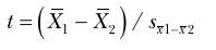
The results of the /-test do not provide the p value directly. Instead, the degrees of freedom and the value of t are used to locate the right /»value in a t distribution table. Sound confusing? Don’t worry. Statistical software packages, including SPSS and R, calculate the p value automatically and list it in the “sig."—or significance—column. Just know that mathematically, t is the observed difference between the two sample means divided by the standard error of the difference between the means.
In notation form, the t value is determined by:
where
X, - X2 is the observed difference between two independent-sample means, and 5»i-x2 *s ^le standard error of the difference between the sample means.
Standard Error
This section introduces a new concept, standard error. Standard error is the standard deviation of the sampling distribution of some statistic (in this case, the difference of means). The sampling distribution of the mean is a special type of frequency distribution. It is the distribution of the means from many different samples of equal size (see Figure 10.2). Putting these definitions together, we can say that standard error is a measure of how much random variation we would expect from samples of equal size drawn from the same population. The concept is similar to standard deviation, but it always applies to a sampling distribution rather than a population or individual sample.
Mathematically, the standard error of the sample mean is calculated by dividing the sample estimate of the standard deviation, i.e., the standard deviation of the sample, by the square root of the sample size.
In notation form, the standard error of the sample mean is:

where
s is the standard deviation of the sample mean, and n is the sample size.
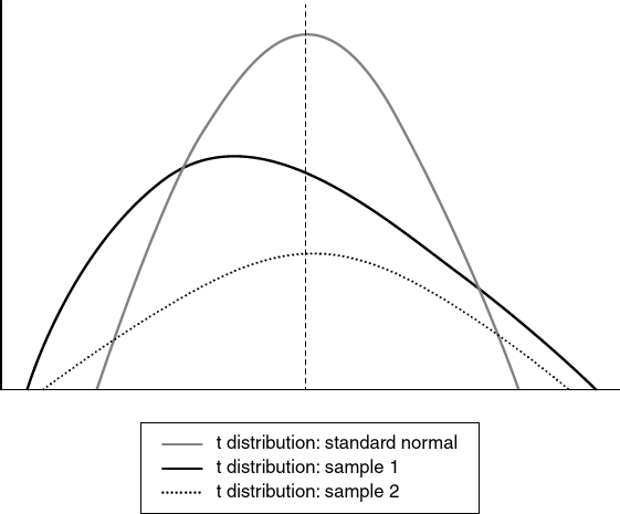
Figure 10.2 The Means of Individual Samples May Differ From the Overall Population Mean and From One Another, but the Distribution of Means From Multiple Samples Tends to Approach a Normal Distribution
Understanding the basic concept of standard error is important, but if you review the equation for determining /, you may notice that it is calculated using the standard error of the difference between the sample means rather than a single sample mean. The concept of standard error is the same whether it is applied to a single sample or the difference between sample means: It is the amount of difference we expect to see between the population mean and a sample mean or, in this case, the difference we would expect to see between the means of two randomly selected samples. However, the way we calculate the standard error of the difference between two sample means is slightly more complicated than for a single sample.
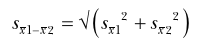
When the samples are roughly equal size, we can calculate the standard error of the difference between the sample means by taking the square root of the sum of the squared standard errors of the sample means. (This is less confusing than it sounds.)
where
srl is the standard error of the mean for the first sample, and is the standard error of the mean for the second sample.

