Basic properties of the model of Seemingly Unrelated Regression Equations
A brief look at estimation and testing within the frameworks of simple and generalised linear regression
To start, let us consider a simple linear regression model. Here is a generic notation of the regression:

where = (Vj,..., vr)' denotes a vector of observations of endogenous variable, dQrxjtj = (.Yjrr')' denotes matrix of observation of explanatory variables, with a single observation containing all xtjs; x, = (xrl,...,xtt)'. For the vector of error terms one may impose standard linear regression assumptions and in particular Gaussian distribution, that is, e ~ N(0, o2IT) we obtain globally optimal estimator of the vector of structural parameters P utilising the Ordinary Least Squares (OLS) procedure:
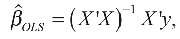
with the covariance matrix:

and its estimates:
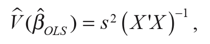
where s2 is an unbiased estimator of o2:

This seminal econometric framework, which almost a hundred years ago was a giant step forward, enriched empirical analyses in many areas, resulting in generalisations in many directions. All econometric models invented so far are derived from simple regression.
One may generalise the simple stochastic structure of the error term in Equation (4.1), assuming that e~N(0, cr2Q). In this case, an elegant and straightforward calculus results from Aitken’s estimator to provide an optimal estimation strategy if the positive definite, symmetric, and non-singular matrix Q [Rr] is known. We denote Aitken’s Generalised Least Squares (GLS) estimator by fla and rewrite it according to our notations:

The unbiased estimator of the covariance matrix is given by:

where is the unbiased estimator of cr2 that utilises the generalised sum of squared errors:

Note that if done coherently, a simple regression is easily obtained from this generalisation by assuming Q = IT.
Aitken’s considerations were formally correct but at the same time useless from an empirical point of view, because (fa as well as ¡’([fa) = cr2 (AAA 'A') requires that the matrix Q is known. In order to make GLS empirically tractable, the estimation scheme requires an inference about matrix Q. This leads us to the Feasible GLS procedure (FGLS). Suppose that the matrix Q denotes the consistent estimator of matrix Q obtained by a researcher prior to making inferences about the structural parameters 0. Given the Q results derived by Aitken, one can generate a consistent FGLS procedure simply by replacing Q by its estimated counterpart:
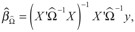
28 Basic properties of SURE
with the small sample approximation of the asymptotic covariance matrix:

and consistent estimator of cr2:

We are not going to discuss all issues concerning simple and generalised linear regressions. The reader can find detailed descriptions together with formal derivations of estimation procedures in many textbooks such as that by Greene (2018).
For the analyses of spatial and temporal disaggregation, we retell an exercise of inference about the linear function of structural parameters. Suppose that the researcher is interested in some linear function y= cp, where is a vector containing coefficients of the linear function under analysis and is known. The inference about 7 is can be easily performed, given estimator

The small sample approximation of the standard error is obtained according to the following formula:
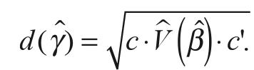
Assuming normality of the error terms in the regression, one may build confidence intervals as well as test hypotheses involving y, just like in the case of structural parameters. For a chosen value ae(0,l), representing the significance level, the confidence interval takes the form

for appropriately chosen two-sided critical value a) that depends on cz, but most importantly on the properties of the estimator
In the case of testing the significance of the restriction imposed on a single linear function /, one may utilise a /-test. Given a chosen value of the significance level ae (0,1) let us consider the following set of hypotheses (null and alternative):
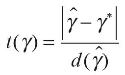
The t statistics of the following form has a distribution with two-sided critical values i? (a):
Suppose that we analyse m linear functions yp...,ym and for each yi=ci[3. Let denote by a matrix containing stacked vectors c,. In the case of the rank of C’ equal to m, one may consider the test of joint restrictions T = C • [3:
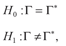
where r*[mT1] = (yj,...,y*„)' contains values of restrictions attached to each linear function. In this case, it is possible to apply the general form of the F-statistic:

