NUTS-2 disaggregation of the Polish GDP: Preliminary analyses within SUREdiag
Polish GDP
Preliminary analyses within SUREdiag
Basic model setting
In this section, we first disaggregate GDP and its growth rate. The results are obtained by an application of the classical linear regression model to the Polish economy. In this approach, the structural parameters of linear regression are estimated. The annual GDP of voivodships (NUTS-2 regions of Poland) or the rate of its changes represent the explained variable, whereas the annual domestic GDP or the rate of its changes fulfil the role of the explanatory variable. The proposed approach consists of estimating the quarterly GDP and its changes for individual regions as functions of the regression parameters. We present the results of GDP estimates and their changes in regions according to empirical series with an annual frequency covering the period from 2003 to 2012. In our approach, diversified GDP deflators were adopted to construct observations of the GDP for the whole country and regions. The whole framework is built on our previous research in this area. The initial version of results presented in this chapter was published as a working paper in Pipien and Roszkowska (2015).
We evaluate our approach in terms of the level of statistical uncertainty associated with the estimation and in terms of the level of spatial diversity of the estimated values. Consequently, in addition to the evaluation parameters, the analysis covers confidence intervals of estimated values obtained from the regression models. Particular attention has been paid to the diversification of GDP estimates, and their changes in regions of Poland during the period of economic slowdown in 2001-2002.
Let us assume that GDP in year t for the i-lh region (voivodship), designated as GDPAR, can be described by the classical linear regression model, where Poland’s GDP in year t is adopted as the explanatory variable (designated as GDPtA N). The regression equation takes the following form:

Let us assume that J’[(iw] denotes the vector of observations on the explained variable, whereas A'[rr2] means the matrix of observations on the explanatory variable with the first column of ones:
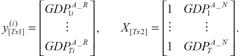
We assume that eti ~ N{Q,cYt), cov(eti,etj) = al eR and assuming that cov(eti, esJ ) = 0, if t ± s. we treat the system as the SUREdiag model, discussed in Chapter 4. Consequently, the regression system parameters in Equation
(5.1) may be estimated using the OLS estimator for each equation separately. Let P OLS = (X'X) 1X' v(/) designate this estimator of the vector of parameters [f! = (POi,pity. The problem of GDP estimation in Quarter n in the z'-th region (denoted by GDP°-R) may be considered as the issue of estimation of linear functions of structural parameters This is because we adopt the following function of parameters as the definition of GDP?-R:

where GDPf-N denotes Poland’s GDP in Quarter n. In accordance with Equation (5.2), we assume that the linear relationship, estimated on the basis of the annual data in regression Equation (5.1), is transferable to the case of data with quarterly frequency. GDPf-R is defined in this manner is subject to unbiased estimation:

The variance of the estimator in Equation (5.1) is provided by the formula:

The approach presented here also allows one to estimate the rate of GDP changes in Quarter n in the z'-th region in relation to the corresponding quarter of the previous year, designated as kGDPf-f

According to Equation (5.4), AGDPf " is a non-linear, differentiable function of regression Equation (5.1) parameters, which is subject to the compliant and asymptotically normal estimation according to the naturally defined estimator:

The asymptotic variance of the estimator Equation (5.5) is provided by the formula:

where

For the estimation of AGDPf-R rate of changes a different approach may be adopted, applying the regression model similar to that defined in Equation (5.1), in which, however, the linear relation between the rates of changes is examined directly. Alternatively, let us thus consider the following regression model:

where AGDPf-R denotes the rate of GDP changes, expressed in percentage, in the z'-th region from year z-1 to year t, whereas AGDPfN denotes the rate of Poland’s GDP changes from year Z-1 to year t. Similarly to the case of Eti in (5.1) we assume that ~ A(0, off, cov(|„, ^) = of and cov(£ti, Q = 0, if t *s. Let = (Z'Z)-1Z'z/(/) denote the OLS estimator of the vector of parameters a(,) = («o,,«!,)', where:
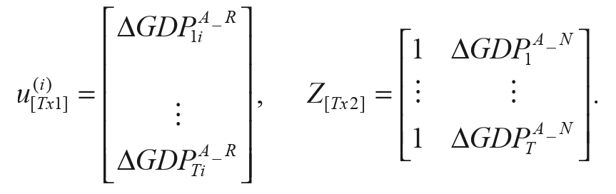
Quarterly GDP changes in an individual region may be treated as linear functions of regression Equation (5.6) structural parameters. Thus, we assume that in Quarter n for the z-th region, the rate of GDP changes in relation to the corresponding quarter of the previous year is expressed by the formula:

The function of parameters in Equation (5.7) is subject to unbiased estimation according to the formula:

The variance of the estimator in Equation (5.8) is provided by the formula:

