Seemingly Unrelated Regression Equations as an example of generalised linear regression
The linear regression Equation (4.1) was generalised in many directions. However, one of the most critical ideas that gave birth to multiequational models, structural equation models, VAR methodology, and others was to analyse a set of regressions as a system. Suppose that we analyse the system of regressions written in the following way:

In Equation (4.2), we analyse a set of endogenous variables and for each i=l,...,n = (ylj,...,yTi')’ contains observations for each explained
variable. Each regression has its individual set of k, explanatory variables. Hence = (xh-xn')' and /?(,) = (^¡,...,(3^)' contains, respectively, observations of explanatory variables in z-th regression and structural parameters. Systemic treatment of a set of regressions in Equation (4.2) requires imposing particular stochastic assumptions on the vectors of
30 Basic properties of SURE
error terms s(,) = (Si,sn)'. Let consider the following set of four basic assumptions:
Assumption 1 : Zero expectation of each error terms:

Assumption 2: Common variance <7 ?•<+«> of the error terms within a particular regression:

Assumption 3: Possible non-zero contemporaneous covariances (and in consequence correlations) between error terms from different regression equations:

Assumption 4: Zero covariances in all remained cases, except those analysed in
Assumption 3:
For each i - for each j - 1...,«, for each t - l...,T, for each s =
we state that:

Let denote the matrix that contains all elements <7?:

According to Assumption 2, we call E the matrix of contemporaneous covariances. In particular Z is the covariance matrix of £., = (e(1,.that groups the row vector of error terms at time t.
In the next step, we stack the observations expressing the system of regression equations in the closed form:

where = (y,»',...,y<">')',£[„rzl] = (e®= (/3(1)and:

with K = kx+ ... + k„.
A simple calculation yields the form of the covariance matrix for the error term £ in Equation (4.3):
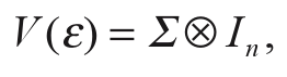
where ® denotes the Kronecker product.1 The form of the covariance matrix of e makes the system Equation (4.3) a generalised linear regression. Based on Z, the Aitken Generalised Least Squares (GLS) estimator of all parameters in the system can be expressed in the following form:

with the covariance matrix of the estimator given as follows:

In a general case, we must estimate the covariance matrix Z prior to the estimation of parameters B. Here we refer to the well-known Zellner (1962) method, and estimate the elements of matrix Z on the basis of the OLS residuals, denoted by £["Mi - (gozs ,...,gozs')'. The FGLS (Feasible GLS) estimator, proposed by Zellner (1962), takes the form:

with the approximated small sample covariance matrix of the estimator:

1 ^(1) *(n) -"-(1) ^(n)
where S = —(£ ,...,£ )'(£ ,...,£ ) is obtained based on the matrix of residuals.
Matrix S' enables to derive estimates of contemporaneous correlations, organised in matrix R of the form:

The considerations stated here should convince the reader of the importance of a single linear regression with a simple or complex stochastic structure. The system of regression Equation (4.2) is in fact the generalised linear regression model that enables one to apply Aitken’s approach.
There are two interesting special cases of Equation (4.2). The first relates to uncorrelated contemporaneous errors, while in the second case, all endogenous variables have the same set of explanatory variables. We denote these special cases as SUREdiag and SUREX respectively.
In model SUREdiag, we impose zero restrictions on non-diagonal elements of the covariance matrix Z, making Assumption 3 much stronger, since Vi, j such: i j,cov^Eti,Etj) = 0. Consequently:

Simple calculus yields the equivalence of Aitken’s GLS point estimator to the application of the OLS estimator for each equation separately:

The difference between an estimation with the use of Bfgls and Bols also concerns the form of the covariance matrices. The diagonal matrix Sdiag = diag(s^,...,sf) should be applied as an estimator of Z = dtag^,

. , , 1 do , ~(O
With .S',7 = —Sols Sols ; = 1,
Basic properties of SURE 33
In case of SUREX, we regress the set of m endogenous variables by the same set of explanatory variables with the observation matrix x[Txk]:

In this case, K = nk. According to the properties of the Kronecker product, one may notice that:

Again, in this case, for any unconstrained covariance matrix Z, we have the equivalence of the point estimates just like in the previous model constraint:

The assumption that for each i the Gaussian error terms £ti in Equation (4.2) are uncorrelated makes the system of equations independent. This case formally refers to the empirical strategy of estimating parameters separately within a particular z-th regression. However, in general, the error terms £tj may exhibit cross-correlations. Non-zero contemporaneous correlations of the error terms in Equation (4.2) define a more ample stochastic structure particularly suitable for formally testing SUREdiag as a particular case. The standard interpretation of non-zero contemporaneous correlations is also used as indicators describing linkages in the variability of related parameters across equations.
Note
1. For matrices J|-M] =(a,7) and B[pxr] =(blj) we define matrix C as a results of the Kronecker product, denoted by C[lpxkr] = A® B, as follows:

We list some useful properties below:

34 Basic properties of SURE

Additionally, for square matrices 4»] and B[pxp}-.


