Empirical results

In Figures 6.1, 6.2 and Tables 6.1 and 6.2, we put results of spatial and temporal disaggregation based on the approach described in Equations (6.1), (6.2), and (6.3). First, we estimated the model based on annual data for the Polish economy, covering the period from 2009 to 2017. Then we estimated logarithms of quarterly NUTS-2 GDP and GDP growth rates over the period IIQ2009 to IVQ2017. Figure 6.1 and Table 6.1 presents plots of estimates of logarithms of quarterly regional GDP (Figure 6.1) and quarterly regional annual GDP logarithmic growth rates (Table 6.1) together with bands of 95% confidence intervals. Tables 6.1 and 6.2 contain numerical values of analysed estimates.

The underlying translation of the relationship between annual macroeconomic indicators in Equation (6.1) to NUTS-2 regions and to more frequent measurements generates spatial and temporal disaggregation of GDP and its growth rate characterised by remarkably high statistical uncertainty. This result is particularly visible in the case of regional GDP growth rates (Figure 6.2) by an enormous range of 95% confidence intervals. Comparing the estimates discussed here with the ones presented in Chapter 5, one notices that the application of a simple growth Equation (6.1) by including other macroeconomic variables generates estimates of regional GDP growth rates much more diverse, indicating substantial economic differences among analysed regions. The price that one must pay for stating such a simple regression like Equation (6.1)

Figure 6.1 Estimated values of logarithms of quarterly regional GDP (per worker) and 95% confidence intervals; see Equation (6.4)

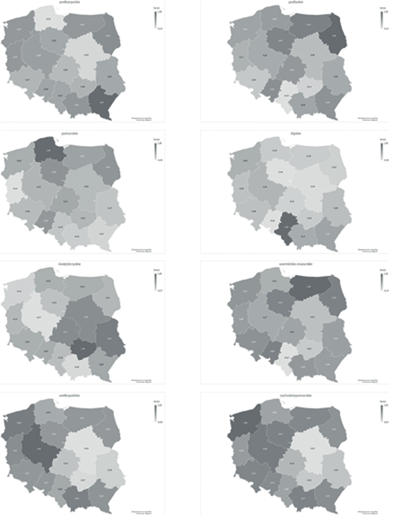
Figure 6.1 (continued)

Figure 6.2 Estimated values of quarterly regional annual GDP (per worker) logarithmic growth rates and 95% confidence intervals; see Equation (6.6)

Figure 6.2 (continued)

Table 6.1 Estimated values of quarterly regional GDP per worker; see Equation (6.4)

	Dolnoslaskie	Kujawsko-pomorskie	Lubelskie	Lubuskie	Lodzkie	Malopolskie	Mazowieckie	Opolskie
2009Q2	3.20	3.07	3.05	3.06	3.01	3.11	3.36	3.11
2009Q3	3.19	3.10	3.09	3.05	3.05	3.11	3.35	3.09
2009Q4	3.22	3.12	3.13	3.08	3.09	3.13	3.39	3.10
2010Q1	3.25	3.16	3.19	3.17	3.14	3.19	3.44	3.19
2010Q2	3.24	3.08	3.09	3.11	3.07	3.14	3.41	3.08
2010Q3	3.22	3.11	3.11	3.03	3.10	3.15	3.37	3.09
2010Q4	3.25	3.13	3.18	3.11	3.17	3.19	3.42	3.12
2011Q1	3.25	3.15	3.22	3.12	3.17	3.21	3.46	3.17
2011Q2	3.23	3.10	3.13	3.04	3.11	3.16	3.42	3.10
2011Q3	3.22	3.15	3.14	3.11	3.14	3.18	3.42	3.13
2011Q4	3.28	3.17	3.19	3.12	3.18	3.21	3.45	3.16
2012Q1	3.28	3.20	3.25	3.14	3.23	3.25	3.45	3.21
2012Q2	3.24	3.17	3.19	3.09	3.18	3.22	3.43	3.14
2012Q3	3.24	3.16	3.18	3.07	3.18	3.20	3.42	3.11
2012Q4	3.28	3.17	3.21	3.13	3.23	3.22	3.44	3.14
2013Q1	3.30	3.24	3.27	3.16	3.26	3.28	3.47	3.23
2013Q	3.30	3.18	3.17	3.09	3.20	3.23	3.43	3.14
2013Q3	3.27	3.19	3.21	3.13	3.22	3.23	3.43	3.14
2013Q4	3.31	3.23	3.23	3.14	3.25	3.25	3.48	3.15
2014Q1	3.32	3.26	3.30	3.19	3.28	3.30	3.53	3.24
2014Q2	3.29	3.19	3.22	3.15	3.21	3.25	3.48	3.19
2014Q3	3.30	3.21	3.22	3.13	3.24	3.26	3.46	3.19
2014Q4	3.37	3.24	3.28	3.16	3.27	3.26	3.50	3.19
2015Q1	3.35	3.26	3.32	3.21	3.32	3.33	3.54	3.28
2015Q2	3.31	3.17	3.24	3.12	3.23	3.26	3.49	3.20
2015Q3	3.30	3.20	3.26	3.14	3.24	3.26	3.48	3.19
2015Q4	3.34	3.22	3.29	3.17	3.29	3.31	3.52	3.22
2016Q1	3.34	3.26	3.39	3.20	3.31	3.32	3.56	3.27
2016Q2	3.31	3.21	3.26	3.15	3.23	3.27	3.51	3.22
2016Q3	3.35	3.23	3.25	3.17	3.26	3.30	3.50	3.22
2016Q4	3.35	3.25	3.30	3.20	3.29	3.29	3.53	3.25
2017Q1	3.35	3.26	3.35	3.20	3.29	3.32	3.56	3.29
2017Q2	3.38	3.24	3.26	3.17	3.27	3.30	3.54	3.26
2017Q3	3.35	3.25	3.27	3.18	3.27	3.31	3.53	3.25
2017Q4	3.38	3.28	3.34	3.21	3.31	3.35	3.56	3.28

Podkarpackie	Podlaskie	Pomorskie	Slaskie	Swietokrzyskie	Warminsko-mazurskie	Wielkopolskie	Zachodniopomorskie
3.07	3.01	3.12	3.10	3.13	3.01	3.06	3.10
3.08	3.03	3.13	3.13	3.09	3.01	3.06	3.10
3.11	3.05	3.17	3.20	3.14	3.05	3.12	3.17
3.20	3.19	3.22	3.23	3.21	3.14	3.16	3.24
3.12	3.11	3.16	3.15	3.13	3.03	3.10	3.15
3.12	3.12	3.19	3.20	3.12	3.04	3.13	3.15
3.15	3.15	3.22	3.27	3.17	3.11	3.16	3.19
3.18	3.18	3.22	3.22	3.23	3.12	3.17	3.22
3.13	3.09	3.19	3.21	3.13	3.04	3.13	3.15
3.17	3.12	3.20	3.25	3.16	3.07	3.14	3.18
3.20	3.18	3.23	3.30	3.20	3.12	3.16	3.22
3.24	3.20	3.28	3.27	3.26	3.18	3.18	3.26
3.17	3.12	3.23	3.25	3.19	3.13	3.16	3.19
3.18	3.15	3.21	3.25	3.17	3.09	3.14	3.15
3.21	3.19	3.26	3.34	3.20	3.13	3.15	3.22
3.27	3.23	3.32	3.31	3.27	3.20	3.19	3.26
3.20	3.15	3.26	3.25	3.19	3.14	3.16	3.17
3.22	3.17	3.25	3.26	3.17	3.14	3.15	3.20
3.27	3.21	3.28	3.37	3.20	3.13	3.20	3.22
3.33	3.27	3.37	3.35	3.28	3.22	3.21	3.27
3.24	3.21	3.29	3.29	3.20	3.17	3.18	3.18
3.23	3.21	3.29	3.29	3.20	3.18	3.18	3.20
3.29	3.23	3.31	3.37	3.22	3.16	3.21	3.23
3.32	3.29	3.37	3.36	3.30	3.28	3.24	3.29
3.23	3.19	3.30	3.29	3.22	3.18	3.17	3.19
3.26	3.20	3.30	3.31	3.20	3.17	3.18	3.24
3.29	3.25	3.32	3.37	3.26	3.21	3.19	3.26
3.32	3.31	3.36	3.34	3.31	3.28	3.24	3.29
3.26	3.25	3.32	3.31	3.21	3.20	3.22	3.26
3.28	3.26	3.32	3.30	3.24	3.22	3.22	3.27
3.29	3.26	3.34	3.35	3.26	3.25	3.22	3.28
3.34	3.29	3.34	3.33	3.29	3.28	3.24	3.31
3.27	3.23	3.31	3.29	3.21	3.21	3.22	3.26
3.28	3.27	3.31	3.30	3.23	3.22	3.23	3.27
3.29	3.29	3.34	3.36	3.29	3.26	3.26	3.28

Table 6.2 Estimated values of quarterly regional annual GDP per worker logarithmic growth rates; see Equation (6.6)

	Dolnoslaskie	Kujawsko-pomorskie	Lubelskie	Lubuskie	Lodzkie	Malopolskie	Mazowieckie
2009Q2
2009Q3
2009Q4
2010Q1
2010Q2	3.6	-28.2	0.9	6.6	2.1	2.0	2.3
2010Q3	3.2	-27.4	2.8	1.9	-2.8	1.6	1.6
2010Q4	3.4	-23.4	1.9	-0.6	0.5	1.9	3.3
2011Q1	0.5	-22.0	2.7	1.5	0.9	1.9	3.2
2011Q2	-0.2	0.8	-21.6	-3.9	-1.1	4.1	2.2
2011Q3	-0.3	1.0	-15.0	-0.2	2.6	1.7	2.3
2011Q4	3.0	1.2	-12.5	2.5	3.4	0.3	3.3
2012Q1	2.6	-0.9	-8.8	4.4	2.5	1.4	1.3
2012Q2	1.0	2.5	3.7	-29.0	0.0	-0.8	3.3
2012Q3	1.4	3.6	2.4	-20.3	1.9	0.4	0.2
2012Q4	-0.1	3.9	4.7	-19.5	1.3	1.8	0.1
2013Q1	1.9	4.8	3.2	-17.8	1.1	0.1	4.7
2013Q	5.2	6.8	4.3	5.0	-18.3	-1.9	-1.3
2013Q3	3.6	1.7	3.1	-2.0	-11.9	3.2	1.6
2013Q4	3.3	0.0	1.8	3.2	-9.6	0.4	4.1
2014Q1	2.5	3.5	2.9	-4.6	-6.7	2.2	-1.9
2014Q2	-1.0	1.0	5.9	-6.5	6.2	-18.3	0.2
2014Q3	2.6	2.2	3.1	7.4	5.1	-15.4	2.2
2014Q4	5.5	6.2	1.3	1.3	7.9	-13.8	0.4
2015Q1	2.4	2.6	1.6	2.1	3.0	-11.5	5.4
2015Q2	1.9	1.1	-1.9	4.7	3.6	3.1	3.6
2015Q3	0.4	2.1	3.8	-3.9	3.6	3.5	5.5
2015Q4	-3.2	1.3	2.7	0.3	1.6	6.5	8.4
2016Q1	-0.6	0.1	2.9	2.2	6.4	1.8	9.7
2016Q2	0.0	-1.8	5.4	0.5	7.2	1.5	5.5
2016Q3	5.1	-1.0	0.8	6.2	3.9	3.8	2.0
2016Q4	1.5	-2.2	4.2	1.4	4.3	2.0	2.7
2017Q1	0.9	-0.8	2.6	2.2	2.6	4.0	1.3
2017Q2	7.0	4.0	1.5	5.7	1.3	6.0	1.3
2017Q3	-0.1	3.6	3.5	0.5	4.5	1.2	5.4
2017Q4	3.1	2.9	1.0	2.0	2.6	0.6	2.8

Opolskie	Podkarpackie	Podlaskie	Pomorskie	Slaskie	Swietokrzyskie	Warminsko-mazurskie	Wielkopolskie	Zachodniopomorskie




-0.5	-2.0	-8.0	0.0	1.3	0.7	-0.1	-0.6	1.2
0.8	1.7	5.0	-32.7	-2.3	-0.4	1.4	1.3	2.0
-0.7	3.8	4.5	-24.1	-1.5	1.9	0.6	1.1	0.3
-0.6	4.0	3.6	-23.1	1.1	1.6	2.4	3.2	5.4
1.5	3.6	-1.7	-10.1	3.0	1.7	0.4	2.0	-0.3
-0.5	4.1	1.1	9.5	-16.8	-2.0	-2.5	2.0	2.0
1.1	-1.5	4.7	9.4	-10.4	-0.8	1.2	2.7	3.6
4.4	-1.7	5.1	9.6	-9.7	-0.5	-0.6	0.3	3.6
6.0	2.4	5.5	-0.6	-7.3	0.4	-2.4	4.5	2.6
4.9	0.4	4.1	-1.8	3.7	-24.0	-0.6	0.5	6.2
2.8	2.8	1.3	-0.3	5.8	-18.3	-1.4	-1.7	0.7
1.3	0.6	1.2	3.3	4.6	-10.8	-0.2	3.9	-0.9
1.7	0.6	3.4	1.9	0.1	-11.5	1.4	0.0	6.0
1.2	4.2	2.4	3.7	2.9	5.2	-19.6	-1.3	0.1
2.5	5.3	4.3	3.4	1.1	7.1	-19.8	-0.1	2.4
2.6	4.3	5.4	0.6	1.4	7.0	-16.7	-1.6	5.4
1.9	4.1	6.5	2.5	6.5	-0.6	-15.5	2.3	3.0
2.6	1.3	4.3	2.7	3.8	6.0	0.1	-28.4	0.0
2.0	-0.4	0.9	2.3	1.4	5.0	2.7	-19.3	0.5
1.0	3.5	2.8	2.1	2.3	3.0	3.2	-17.4	-0.5
-0.2	-0.7	-1.6	4.2	3.3	5.4	2.2	-14.2	1.5
2.7	1.6	-1.3	5.7	3.6	3.5	-0.9	2.4	-21.5
2.5	3.4	2.8	3.3	3.8	-0.6	3.6	2.4	-15.3
2.3	2.4	-0.3	2.3	2.7	3.6	3.0	5.8	-9.6
-44.8	1.9	0.0	1.6	5.4	3.7	3.3	-2.1	-10.2
-44.8	4.1	3.9	-1.7	2.7	0.6	6.6	0.2	3.5
-42.5	2.4	1.8	-0.8	3.4	1.8	1.0	3.3	7.2
-36.6	3.0	0.0	1.6	3.0	2.9	0.7	0.9	4.0
-2.9	-22.0	1.8	2.8	-0.6	3.7	0.9	5.3	1.3
-0.3	-18.0	0.2	5.8	1.3	3.4	-0.4	9.7	2.7
1.7	-13.4	0.4	6.1	1.4	2.3	0.3	1.8	0.9

is statistical uncertainty and huge variability of economic fluctuations among regions. Analysing path of GDP annual logarithmic growth rate (Figure 6.2), we report very stable growth for the Mazowieckie region, while in the cases of the Lubuskie, Lubelskie, and Opolskie voivodships, a possible economic recession may reach a 20% contraction of the quarter GDP or even more. Our results clearly illustrate how enforcing diversity of regional estimates of GDP and its growth rates produces an explosion of statistical uncertainty inherent in the approach.

Consequently, the researcher obtains a vague picture of regional economic growth.