Stage Eight. Experimental Study of Systems

Often the missing information about the system can be obtained only from the system itself by conducting a specially planned experiment. The information contained in the experiment protocol is extracted, subjected to data processing, and converted into a form suitable for inclusion in the system model. The final action is model correction which includes the obtained information in the model. This section explains various measuring scales and correct processing measurements.

Experiment and model. Often the missing information about the system can be obtained only from the system itself by conducting a specially planned experiment. The information contained in the experiment protocol is extracted, subjected to data processing, and converted into a form suitable for inclusion in the system model.

The final action is the model correction which includes the obtained information in the model.

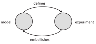
It is clear that an experiment is needed to improve the model. It is also important to understand that an experiment is impossible without a model as they follow the same cycle (Figure 5.9). However, rotation along this cycle does not resemble a rotating wheel, but a rolling snowball, with every turn it becomes more and more weighty.

Experiment and measurements. Various experiments can be described simply by their classification. If we do not interfere in the course of events but only register what happens at the inputs and outputs of the system of interest to us, then the experience is called a passive experiment (or observation). If we not only contemplate (and record) what is happening at the inputs and outputs but also affect some of them (some deliberately maintaining unchanged, while others changing properly), the experience is called active (or controlled) experiment. Like any classification, this only approximates reality. In absolutely pure form, these two experiments are impossible: active — because all the inputs and outputs cannot be controlled (some are even unknown), and passive — because every measurement and observation is an interaction, and it is impossible not to interfere with the result. The closest real, close to ideal, experiments are active laboratory experiments and passive observations in astronomy, history, archeology, psychology, etc.

Another important classification is dividing experiments into direct and indirect. A direct experiment is an observation of the characteristic that interests us (e.g., the gain of young animals can be measured by daily weighing). Sometimes the characteristic we are interested in cannot be directly measured, but there is an observable quantity associated with it; from the observations, we can extract the information we need; this will be an indirect observation (e.g., some actions of a mother can be judged on the strength of maternal love; those of prices on the cost; of blood pressure on the state of the cardiovascular system). The division of measurements into direct and indirect is important because they need to be treated differently, even if they are described using the same scale.

The results of the experiment are recorded in the form of a protocol of observations. This record is not the experiment itself but the description of its result, that is, its model. Understanding the term “language” widely, we can say that the protocol of observations is a record of the results of the experiment in some language. The variety of experiments is such that one language is indispensable; there are several such languages, called measuring scales. You should familiarize yourself with them because, in practice, you will

have to deal with data processing on different scales, and this should be done differently for each scale. As in any language, incorrectly constructed phrase loses its meaning, and incorrectly transformed experimental data do not carry the expected information.

Measuring scales. On the example of measuring scales can be traced the phenomenon characteristic of all languages (remember the discussion of language models in Chapter 3): starting with a universal but low-informative language, you can, including by attaching additional information to it, get more and more informative languages up to the most mathematized.

1. Scale of designations (nominal, classification). In the section on abstract models in Chapter 3, it was noted that the simplest model of diversity is classification. It is the basis of the scale of names. The measurement in this scale is to observe the classification characteristics of the object to determine to which class it belongs and to record it using a symbol denoting this class.

Family names, diagnosis of diseases, number of houses and cars, players of sports teams, names of colors, addresses, etc. are examples of observations in the nominal scale.

Let к classes be introduced: A,, A,, ..., A_k (A_s is the name of s-th class). Let the objects x_1; x₂, ..., x_N be successively observed (their set is called a sample, N is the sample size). With respect to each x, (i = 1... N) is concluded to which of the classes A,, ..., A_k it refers (x_f e A_s). The result is a protocol of observations.

Since the only relationship defining the scale is the equivalence relation (the object either belongs to this class or not), the only admissible operation on the data in this scale is a match check, that is, a check for coincidence. This operation is represented by the special Kronecker symbol 8,,j = {1: x, = x; 0: X; x }, that is, the coincidence of two different observations (belonging to the same class) is denoted by one and the mismatch is zero. With the results of this primary processing, you can perform secondary processing. For example, the number of observations in one class with xi is n, = X, 8_tj, and the relative frequency of this class will be /t,77V, the number of the most populated class /_max = {arg(max n,)}; you can use different statistical procedures that use relative frequencies (e.g., the y² test).

It is possible to compare the data in the nominal scale obtained by different researchers only if they used the same division into classes (the number of classes and the boundaries between them must coincide). Only the names of classes and the order of their enumeration can differ as they do not violate the natural structure of the data.

Once again, we recall that no operations on {x,}, except for the comparison operation 8_t), can be done; otherwise, the result will not be valid. For example, if you know that there are a hundred houses on the street, it is wrong to say that the geographical middle of the street is about the 50th.

2. The preference scale (ordinal, rank). If you enter an additional relation of the order between the classes of the nominal scale (preference; denote it by a symbol >), you get a new and enhanced information sense of the scale, called ordinal or ranking.

Examples of observations recorded in the ordinal scale include army and official ranks, school grades, magnitude of earthquakes (Richter scale), hardness of minerals (Mohs scale), wind strength (Beaufort scale), and prizes in competitions.

The valid transformation <5,-, (note at once that the valid transformations for weaker scales are also valid for stronger scales, but not vice versa) is now complemented by the preference check operation C,_;: = {1: x_f >- xf,

0: x,- ax-}. Thus, the primary data processing in the ordinal scale consists of two valid transformations: 8_tj and C_tj. The use of other operations will lead to misunderstandings. An example is an unsuccessful attempt to account for the “average school score” when entering universities. In this failed experiment, the scores were treated as numbers and added up. The addition operation in the ordinal scale is invalid and gives a meaningless result. The experiment had to be canceled.

With the results of the primary processing (binary numbers), you can produce a suitable secondary. For example, you can define the number of observations x, in an ordered series of all observations: R_j = Zf C,_;. This number is called the rank of the i-th object (hence, there is another name for this type of scale, rank). Other uses of the numbers Sg and C_tj are possible: in addition to finding frequencies and modes (as for the nominal scale), it is possible to determine the sample median (i.e., the observation with the rank closest to the number М2), to divide the whole sample into parts in any proportion, to find the sample quantiles of any level p,0 1 (i.e., observations with the rank /?,, closest to the value of N_p), to determine the rank correlation coefficients between the two series of ordinal observations (r₅ Spearman, r Kendall), and to build other statistical procedures.

A few additional remarks on ordinal scales.

Various preferences are ordering in the presence of standard reference samples (e.g., the Mohs scale is based on ten specific minerals of different hardness), with fuzzy samples (wind force scale, school grades) in the absence of samples (sports, music competitions).

In addition to the scales of perfect order, unambiguously determining preferences (sequence numbering, military ranks, etc.), there are scales of quasi-order, when some elements of the ordered series are indistinguishable (mother = father >- son = daughter; uncle = aunt A brother = sister), as well as scales of partial order, when there are incomparable pairs of classes (e.g., in sociological studies, the subject is sometimes unable to assess what he likes more — checkered socks or canned fruit, bicycle or tape-recorder, reading or swimming, etc.).

In ordinal scales, there is no concept of distance between classes, so any transformations that preserve order (“monotone”) do not affect the information contained in the data. (Soldiers hanging on the shoulder straps a star and all higher ranks adding an asterisk will be prettier, but the essence does not change.)

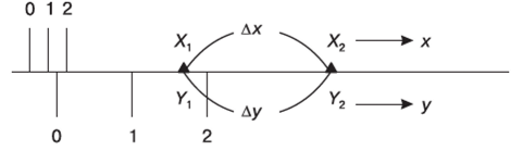
3. Scale of intervals (differences). If the ordering of objects can be done so precisely that the distances between any two of them are known, then the measurement will become noticeably more informative than that in the order scale. It is natural to express all distances in units, although arbitrary, but the same throughout the length of the scale. This means that objectively equal intervals are measured by the same segments of the scale wherever they are located (Figure 5.Ю).

As a result, it turns out that in our new scale, scale of intervals, the origin and the unit of interval length of the interval are arbitrary (ДуДх = const). Examples of observations recorded in the interval scale:

- Temperature (Celsius, Fahrenheit, Kelvin scales);

-chronology (from the birth of Christ, from Muhammad’s move to Medina — 622years later, from the Imperial dynasty in China — 5000years earlier);

- altitude (from sea level; Holland almost all has a negative height).

The only new valid primary processing operation on the data in the new scale is subtraction, that is, determining the interval between two counts. For example, if we say that the temperature has doubled when heated from 9°C to 18°C, for those who are accustomed to using the Fahrenheit scale, this will sound very strange since on this scale the temperature will change from 48.2°F to 64.4°F. The division operation for this scale is also not valid. Only intervals make sense of real numbers. Using them (secondary processing), it is already possible to perform any arithmetic operations, as well as statistical and other procedures.

4. Scale cyclic (periodic, differences). There is a special kind of interval scale which is characterized by the fact that it is closed on itself, that is, after passing a certain period, its values are repeated. Examples include angular directions from a central point (compass scale, wind rose), time of day (clock face), phase of periodic oscillations (in degrees or radians), and geographic longitude (in degrees).

Everything said about the interval scale applies to the cyclic one. To avoid misunderstandings, note that the addition of hours is not the addition of the timestamps themselves (which is an unacceptable operation), but the addition of time intervals between the origin and a clock, that is, secondary processing. We must also remember the conventionality of the start of the countdown (e.g., when switching to winter time, or crossing the date line). This scale is also called the scale of differences as it is invariant to shift to an interval, called the period of the scale.

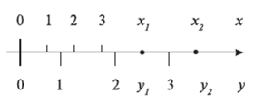
5. Scale of ratios. Introducing a defining relationship gives additional gain measurements. We demand that not only the ratio of the values of the same interval in different scales were constant, wherever this interval may be (that is typical for the scale of intervals), but that the ratio of the values of the same value measured in different scales were also constant, whatever place this value may occupy in reality (see Figure 5.11): x/y, = const, / = (1,... N).

The resulting scale is called the scale of ratios. Although the unit of measurement remains arbitrary, the zero mark becomes absolute and immovable.

Examples of quantities whose nature corresponds to the scale of relations are:

- length (cm, feet, yards, miles, etc.);

- weight (kg, pounds, tons, etc.);

- volume (m- barrels, liters, etc.);

- money (rubles, dollars, euros, yen, etc.).

Data in the scale of ratios become numbers to an even greater extent: in the primary processing, any arithmetic operations make sense, and the same can be done in the secondary processing.

6. Absolute scale. The previous “numerical” scales (of intervals and ratios) had degrees of freedom: intervals—two (arbitrary zero and unit), and relations—one (fixed, immovable zero and arbitrary unit). It is characteristic that the “numerical” capabilities of the data in these scales were limited: in the interval scale, only the operation of the difference, and in the scale of ratios, all arithmetic operations.

Consider a scale that has both absolute zero and absolute unit. This scale has no degrees of freedom, and it is unique. These are the qualities of the numerical axis, which is naturally called the absolute scale. An important feature of the absolute scale is that the data values in it do not have dimensions, names, and its unit is absolute (“item”). This gives the data in this scale a special status (in English they are called pure numbers) — with them you can perform operations that are not valid with named numbers. (Record 2 cm² is valid, but 3^2cm is meaningless.) They can be used as an indicator of the degree, the base of the logarithm, and any trigonometric and other transcendental transformations are allowed for them.

The numerical axis is used as a measuring scale when counting objects, and an auxiliary means is present in all other scales. The internal properties of the numerical axis, for all its apparent simplicity, are diverse and complex — the theory of numbers has not exhausted them to the end. Some dimensionless numerical relations, found both on the axis and in nature, cause amazement and admiration: prime numbers, Fibonacci numbers,

harmonic relations of sounds and sizes, laws of the theory of dimensions and similarity, quantum regularities, etc.

The final table of the basic measuring scales. The six measurement scales discussed above do not exhaust the diversity of languages in which we can talk about the diversity of reality. However, they are basic: the remaining scales are derived from them taking into account some third-party specific conditions. Table 5.2 summarizes some of the important features of the basic scales.

TABLE 5.2

The Final Table of the Basic Measuring Scales

Type of Scale

Defining

Relations

Equivalent

Transformations

Permissible

Operations

Secondary

Processing

Examples

Designations,

nominal,

classification

Equivalence:

Renaming and reordering

Kronecker

symbol

6₉=ll:x, = xfi0:

Xi*Xj)

Calculation of relative frequencies and their processing

Names, numbers of cars and houses, symbols

Reference, ordinal, rank

Same plus preference: =,>-

Not changing the order,

“monotonic”

Same (fy), and comparison function:

C,j = (1: ■*, yxj,

O-.x^Xj)

Same, and

calculation

of ranks: R,

- yxr 4 S’

quantiles

Orderings, school marks, enumeration

Intervals,

differences

Same, and constancy of intervals ratio:

MAAv = =const

Y = a.x + b, a > 0, b e R

Same, and calculation of intervals:

S_ip C_f and

^&9 = ^xij-Xj

Arithmetic

operations

over

intervals

Temperature, chronology, height of locality, latitude

Differences

cyclic,

periodic

Same, and periodicity:

=. >-,

AxAx = =const; and

у = .v + b hit

Same, and periodicity

Same as above

Same as above

Clock, compass, seasons, phase of oscillation

Ratios

Same, and constancy of ratio of measurements: =. >-,

AxAx = =const, and

ylx = const

у = ax + 0

All arithmetic operations

All

arithmetic

operations

Length, weight, volume, mass, area, money

Absolut

Same, and absolute zero and unit

Scale is unique: numerical axis

Any arithmetical and

transcendental

operations

Any

operations on numbers

Calculation of something, of proportions, basis of other scales

Other scales. Measurement practice in various activities has led to the desirability of introducing scales that are different from the basic ones. Considering the purposefulness of this text to professionals of any specialty, we restrict ourselves to a brief listing of the most commonly used modifications of the measuring scales, so that if you wish you can find more detailed information.

Measurements of continuous quantities are very common, and their values are inevitably recorded with finite accuracy and rounded. A special case is represented by scales when a finite number of digits is determined not by the digit capacity of the recording device, but by the accuracy class of the measuring device, when it is pointless to increase the number of digits. Both types of scales, as opposed to integer discrete scales, are called discretized. Data processing in discretized scales has a number of features.

Another practically important class of scales is nonlinear. The intervals of these scales do not meet the conditions of additivity, that is, the “price” of a unit division of such a scale depends on which part of the scale this division exists. Examples include quadratic, logarithmic, exponential scales, “probabilistic paper”, and many nomograms.

Attempts are made to fill the gap between “weak” (nominal and ordinal) and “strong” (numerical) scales: the hyperorder scale and the Churchman-Ackoff scale.

In principle, each researcher can build their own measuring scale to better represent their results. It is very important to emphasize that each scale must be accompanied by a list of permissible primary processing operations that are specific to this scale.

So far, we have discussed scales based on a clear classification: an element either belonged to a class or did not. Real life has led to the need to consider cases where the requirement of strict equivalence is not met, that is, when an element can simultaneously belong to two or more classes. Two approaches have been developed to describe such situations.

The first is based on the theory of fuzzy (vague) sets. In this theory, class membership is described by the membership function, which characterizes the degree of confidence with which we attribute an object to a class. For example, to what extent does a 40-year-old belongs to the “young people” class, and to what extent to the “middle-aged”? In this theory, the measuring scale is the scale of values of the membership function.

The second approach is to consider that the probability distributions of the variable to be classified may overlap. It means that the measured value may belong to either one of the classes with corresponding probability. When deciding whether a variable belongs to one or another particular class, we dissect the range of values of the variable into distinct classes, resulting in error probabilities (Figure 5.12). Processing of random variables is done in mathematical statistics.

In carrying out the experiment, the information obtained depends on numerous factors:

a. how the experiment was organized, what values and in what order the managed variables were assigned;

b. what are the noises, errors, and distortions of the observed variables;

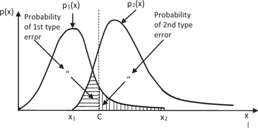
FIGURE 5.12 Statistical classification.

c. to what extent are fair the assumptions put in our model of the system under study;

d. what are the methods and algorithms for processing the experimental data.

The significance of these factors varies in different experiments; therefore, special theories have been developed on how to improve the quality of conclusions depending on a particular combination of factors. If necessary, you can refer to the appropriate ones:

- theory of interpolation and extrapolation;

- design of experiment;

- nonparametric statistics;

- robust statistics methods;

- optimization theory;

- search and strengthen patterns.

These keywords can be found in the catalogs of the necessary literature.

Why such details? Indeed, the proposed text is addressed to a wide range of readers: according to the author, knowledge of the basics of applied systems analysis is necessary, at least useful, for specialists of any profession. It is clear that if it comes to experiments, measurements, and processing of the data, especially in difficult conditions, it is rare for one person to perform all operation, and he will turn to specialists to get the final result.

However, practice shows that in trying to make it easier for themselves, experts often neglect some of the subtleties of data analysis, sincerely believing that they are insignificant. A typical example is the often used “digitization” of qualitative data — classes in ordinal and nominal scales are assigned numbers, and then these numbers are processed not as symbols, but as numbers, using arithmetic operations. But these are unacceptable operations for these scales! Another example is the weakening of data to bring it to monotony. In a table with disparate data, the strong scales are coarsened to the weakest (usually ordinal), so that the experiment protocol becomes single-scale, which facilitates processing. Unlike digitization, it is not the imposition of alien information, but the rejection of some useful information. This also reduces the quality of the conclusions.

The main task in the presentation of this stage is to direct the attention of the user of experimental services to check whether the use of invalid operations happened during the processing of data. For example, all numeric scales operate with numbers. But we already know that the numbers in the scale of intervals, ratios, and absolute should be treated differently. When accepting an order, it is recommended to check if there are any invalid operations in the processing algorithm.

Another important point to keep in mind is the coordination of the information power of the measuring scale with the information potential of the observed phenomenon. The stronger the scale, the greater the “information harvest” from the experiment. Therefore, each experimenter tries to use as strong a scale as possible. However, it is impossible to consider an observation with an arbitrarily set zero as belonging to the scale of ratios. Thus, when a direct observation is desirable, the scale of measurement makes you stronger, but not stronger than the very nature of the phenomenon.

The matter is even more complicated with indirect observations. The observed value, indirectly related to the unobservable phenomenon of interest to us, can belong to any scale, including the strongest scale; whereas the information potential of the phenomenon itself can be significantly lower. How to process such experimental data? The answer is that in the processing of indirect data, no matter how strong the scale they are recorded in, do not use operations that are unacceptable in the scale corresponding to the nature of the phenomenon under study. We will give one serious and two humorous examples.

Let us try to measure the power of a mother’s love. This characteristic cannot be directly measured, but it is possible to record the number of rewards and punishments that a mother gives a child per day. The number of slaps and candies are fixed in the strongest, absolute (!) scale. The hypothesis is the assumption that these values are monotonously connected with the power of the mother’s love for the child. But if one mother has the appropriate characteristics twice as better than the other, it is wrong to conclude that she loves her child twice as much; we can only say that she loves more because the power of love belongs to a qualitative, ordinal scale.

The second example is taken from medicine. The rate of precipitation when sodium citrate is added to a test tube containing blood is taken as an indicator of the intensity of the pathological process; the rate of precipitation is measured in millimeters per unit time. This idea is based on the fact that an increase in the intensity of inflammation leads to an increase in the content of globulin, which increases the rate of precipitation. The functional form of this relationship is unknown, and for different patients, it is different and nonlinear: the change in the proportions of sodium citrate or of deposition time leads to disproportionate changes in the elevation of sediment. Now, let for one patient medicine A led to a decrease in sediment (for 10 minutes) from 75 to 60 mm, and for another medicine В from 65 to 55 mm. Both the deposition time and the sediment height are measured in the scale of ratios. From here, it is impossible to conclude that the drug A is more effective since it led to a decrease in the sediment by 15 mm and the drug В only by 10! The intensity of inflammation belongs to the ordinal scale.

The third example is the test of mental abilities, which measures the time spent by the test subject to solve the test problem. In such experiments, although time is measured in a numerical scale, the measure of intelligence belongs to the ordinal scale.

Thus, the main pathos of the presentation of this stage of systems analysis is aimed at ensuring that, if necessary, the experimental study of the system with which you have to work, whether you will carry out experiments or will order them to others, would check if the experimental data are processed correctly. A typical situation is the widely used counting ratings case.

Questions and Tasks

1. What are “active” and “passive” experiments?

2. What is the difference between direct and indirect measurements? How should we take into account the difference between them when processing experimental data?

3. Have you learned the characteristics of the basic measurement scales? For example, have you noticed that quantitative scales differ in how you define the origin and units of measure?

4. Why should data from different measurement scales be treated equally always?

5. Try to identify the scales in which entries are made in each column on the page of a student’s gradebook.