Basic Equation

Consider an assembly comprised of two identical components, #1 and #2, subjected to different temperatures and supported by a plurality of identical supports (legs). In Figure 3.11, an arbitrary segment of a multileg assembly is shown. There might be many similar segments to the left and to the right of the one depicted in this figure.

The longitudinal interfacial displacements of the bonded components (“adher- ends”) can be sought in an approximate form as follows:

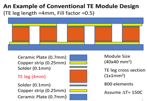
FIGURE 3.11 An example of a conventional ТЕМ design.

Here, a is the CTE of the component material, Д/, and Дt₂ are the changes in the component temperatures (from the manufacturing to the operation temperature),

?i_: = -—— is the axial compliance of each of the two identical components, £, and v,

are the elastic constants of their material, /?, is component thickness, T(x) = jt (!;)<$;

о

is the induced force acting in the cross sections of assembly components in the given cross section, x(x) is the interfacial shearing stress, and к, is the longitudinal interfacial compliance of the component. The origin of the coordinate x is in the midcross section of the bonded region. The first terms in formulas (3.7) are unrestricted thermal displacements. The second terms are due to the elastic displacements caused by the thermally induced forces T(x), assuming that these forces are uniformly distributed over the given cross section. The third terms are, in effect, corrections to this assumption. They consider that the displacements of the point located at the interface, where the thermal forces are applied, are larger than the displacements of the inner points of the cross section. These terms are based on an assumption that the corrections in question can be evaluated as products of the (so far unknown) distributed interfacial shearing stress acting in this cross section and the (position- independent) interfacial compliance of the given assembly component. The total interfacial compliance of the assembly is due to both the components and the bond

and can be evaluated using the recommendations in [11, 12]. For small — values (say,

below 0.25) the interfacial compliance of the assembly components loaded on one of

h £

their long sides can be evaluated as к = —, where G =-is the shear modulus

⁶ 3 G 2(1+ V)

of the material. For the assembly components (e.g., such as the bonding layer) loaded on both sides in an antisymmetric fashion, the factor 3 in the denominator of the previous formula for the interfacial compliance can be omitted. In another extreme

/; 3 — v /

case, for large — values (say, above 0.5), the expression к = ——— can be obtained for the interfacial compliance [18]. Calculations carried out for typical electronic and photonic assemblies indicate that the compliances calculated for the — ratios of

h

0.25 and 0.5 might not be very much different, and therefore, if the actual у ratio falls between the above values, the compliance of the material of interest can be computed by using linear interpolation between its compliance computed for 0.25 and 0.5 aspect ratios. The condition

of the compatibility of the interfacial displacements (3.7) results in the following equation for the interfacial shearing stress t(.v):

where the total compliance к = к₀ + 2к, of the interface can be calculated as the sum

h

of the interfacial compliance k₀ = —— of a buffering (bonding) layer, if any, and the

G₀

two bonded materials. Here, h₀ is the thickness of the buffering layer and G₀ is the shear modulus of its material. From (3.9), we find by differentiation:

For the ith support (leg) in Figures 3.3 and 3.4, this equation could be written as

The solution to this equation can be sought in the form:

The constant В is the particular solution to the inhomogeneous equation (3.11), the second and the third terms (containing hyperbolic functions) provide the general solution to the corresponding homogeneous equation, C, and I), are constants of integration, and к is thus far unknown parameter of the interfacial shearing stress. Since the interfacial shearing stress T(x) can be evaluated as the derivative of the distributed axial force T(x) i.e., x(x) = T'(x), equation (3.12) yields

Introducing the expressions (3.12) and (3.13) into the equation (3.11), we conclude

that this equation is fulfilled, if the relationships к = В = take place.

v к 2K

Equation (3.12) must satisfy the boundary conditions (Figure 3.11) 7) (—/) = 77-ь Ti(l) = Tj. These conditions indicate that the distributed force T(x) in the bonded /th region changes from 7}-_: to T_h when moving from the left end x = -I of this region to its right end x= l. These boundary conditions, solution (3.12), and the formula for the В value yield

Then, solution (3.12) results in the following expression for the distributed force acting within the /th bonded region:

The distributed interfacial shearing stress can be found by differentiation:

The first terms in the right parts of formulas (3.15) and (3.16) are due to the local thermal expansion (contraction) mismatch of the component materials, and the second and the third terms are caused by their global mismatch. It is the global mismatch that results in the forces applied to the bonded regions from the unbonded regions of the assembly.

Theorem of Three Axial Forces

From (3.16), we obtain the following expression for the interfacial shearing stress acting in the / + 1 leg:

The following condition of the compatibility for the longitudinal displacements at the boundary of the bonded and unbonded regions should be fulfilled:

The left part of this condition is the difference in the longitudinal interfacial displacements of the assembly components at the bonded region at its boundary with the unbonded portion. The right part is the difference in the longitudinal displacements of the assembly components at the unbonded portion at its boundary with the bonded region. Introducing the expressions (3.16) and (3.17) into the condition (3.18), the following equation for the forces 7)__b 7), and T_M can be obtained:

where

The recurrent equation (3.19) has the form of (and is based on the same reasoning as) the well-known theorem of three (bending) moments in the theory of continuous beams lying on separate simple supports (see, for example, [18]) and could be called therefore “theorem of three axial forces.” A similar equation has been obtained earlier for the “piece-wise continuous” inhomogeneous bonding layer in a bimaterial assembly [36], that is, for an assembly with no unbonded regions. After the forces Tj-i, T_h and T_i+l are determined, the shearing stress can be found by formulas (3.16) and (3.17). Equation (3.19) can be actually used in the same fashion as the “theorem of three moments” is used in structural analysis of long beams lying on simple supports, namely, by moving, say, from left to right, forming this equation for three sequential axial forces, solving it, and then evaluate the interfacial shearing stresses. Examine several special cases to make sure that the previously obtained formulas for these cases can be obtained from the more general “theorem of three axial forces.”

Special Cases

Homogeneously Bonded Assembly

In this case, one should put 1.7]_, =T_M =0.f_i = f. and equation (3.19) yields [12]

If, in addition, the kl product is significant, such as the assembly is long and/or stiff,

then f = To ⁼ ———. The maximum interfacial shearing stress can be found in this

case as

For a long and/or stiff assembly, tanh kl can be put equal to one and therefore

Assembly Bonded at the Ends (Two-Legged TEM)

By putting 7).| = T_M =0,fi=T, we obtain from equation (3.19) [23]

For the interfacial shearing stress, formulas (3.16) and (3.17) yield

The maximum shearing stress can be found as: t_max = т(/) = т«,%(к(), where т_м = is the interfacial shearing stress at the ends of an infinitely large assembly

• 2Ai
• (or a two-legged assembly with very short-and-thick legs), and the function

considers the effects of the finite values of the product kl and the ratio —. The function X(kl) is tabulated in Table 3.1.

As evident from the computed data, the function %(/:/) can be put equal to 1 for kl values exceeding 4.

TABLE 3.1

Function %(/r/) that Determines the Effect of the Finite Size of the Assembly and the Bonded Regions in it on the Maximum Shearing Stress

TABLE 3.2

Function X_m(kl) that Determines the Effect of the Finite Size of the Assembly and the Bonded Regions in it on the Maximum Shearing Stress

Midportion of a Long Multilegged Assembly

By putting in equation (3.18) T,. =Tj = T_M = T, we obtain: f = „(£/), where

2A,j

the factor

is tabulated in Table 3.2. As evident from the calculated data, this factor can be very small, when the ratio L/21 is significant, such as when the leg spacing is large, no matter how large or small the product kl is. This behavior is quite different of the behavior of the two-legged assembly. Clearly, when the force T in the midportion of the assembly is small, the maximum interfacial shearing stress at the assembly end will be low as well.

The maximum interfacial shearing stress at the end of the assembly can be computed as x_nm = kT tanh kl, where T the axial force is expressed by formula (3.23) and the hyperbolic tangent tanh kl considers the effect of the finite size of the bonded area on the maximum interfacial shearing stress.

TEM Designs in Figures 3.11 and 3.12

Let us apply equation (3.19) to the five-legged structures (designs) shown in Figures 3.11 (conventional design with thick-and-long legs) and 3.12 (novel UCSC design with thin-and-short legs). Going in this equation from left to right, putting sequentially i = 1,2,3,4 and considering the symmetry of the structures in question with respect to their mid-cross sections, we obtain the following two equations for the forces 7j and T₂ acting in the spans between the two peripheral legs (on each side of the assembly) and between the second and the third legs, respectively (Figure 3.13):

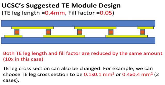
FIGURE 3.12 UCSC ТЕМ design with thinner legs (in our analyses, the upper plate is component #l and the lower plate is component #2).

Since the right parts of these equations are the same, the forces 7| and T₂ have to be related as

From one of equations (3.27) and equation (3.28) we find: where

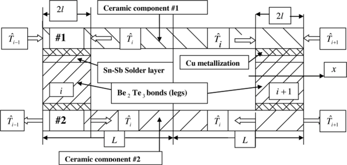
FIGURE 3.13 A segment of а ТЕМ structure.

is the determinant of the system of equations (3.27). The forces 7] and T₂ will be equal if the condition t - c = s takes place. This condition is fulfilled for a long assembly

with a continuous bond, when tanh kl = coth kl = 1 and — = 1.

2I

Equation (3.29) indicates that the induced forces Г, and T₂ will be small and, hence, the induced thermal stresses will be low as well, if the t = tanh kl value is low (short bonded areas with highly compliant interfaces) and/or if the determinant D is significant. The latter condition takes place, as one could see from equation (3.30), if

the span s = Akl f- lj is large. With low t=tanh kl values, such as with low kl values,

this relationship will take place when the ratio is significantly larger than unity.

Consider now a numerical example for the designs in Figures 3.11 and 3.12.

Input data:

The difference in temperature between the hot and the cold components is ДГ = 130°С.

Calculated data:

• Axial compliance of one ceramic component:

• • Interfacial compliances for an infinitely long assembly:
• - Ceramic component:

- Copper layer:

- Solder layer:

- Be₂Te,bond (leg):

Total:

• Parameter of the interfacial shearing stress:

• Maximum interfacial shearing stress:

This stress is well below the yield stress in shear for the solder material that can

be assessed as

Let, for example, the length of the assembly is 2L = 20 and the thickness (dimension in the horizontal direction) of each leg is 21 = 1.0 mm, so that the — ratio is — = 10. Other i nput

data are the same as in the table. The axial compliances X, of each of the ceramic components, and the interfacial compliances к, and K_s of the ceramic components and of the solder layers are not different of those previously calculated. The other computed data are as follows:

• Interfacial compliance of one of the copper layers:

• Interfacial compliance of the leg:

• Total interfacial compliance:

• Parameter of the interfacial shearing stress:

The product kl = 0.4771 x 0.5 = 0.2309

• Maximum interfacial shearing stress in an infinitely long assembly:

• Factor that considers the role of the kl value and the length ratio —:

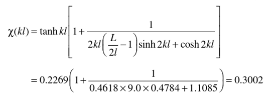21

• Maximum shearing stress

This stress is only 44.0% of the stress in a long assembly with a homogeneous bond. The midportion of a long multilegged assembly can be addressed by putting T-i =fj=f_i+i=f in equation (3.19). Then, we obtain:

where the factor

TABLE 3.3

Function %,„(&/) that Determines the Effect of the Finite Size of the Assembly and the Bonded Regions in it on the Maximum Shearing Stress

is tabulated in Table 3.3. As evident from the calculated data, this factor can be very small, when the ratio Ы21 is significant, such as when the leg spacing is large, no matter how large or small the product kl might be. This behavior is quite different of the behavior of the two-legged assembly (see Table 3.1 data). Clearly, when the force T in the midportion of the assembly is small, the maximum interfacial shearing stress at the assembly end will be small as well.

The maximum interfacial shearing stress at the end of the assembly can be computed as

where T the axial force is expressed by formula (3.31) and the hyperbolic tangent tanh kl considers the effect of the finite size of the bonded area on the maximum interfacial shearing stress. With the input data from the previous examples, formula (3.32) yields

The induced forces in the midportion of the assembly are The maximum interfacial stress is

This stress is significantly lower than the stress in a two-legged assembly: it is only 5.3% of the stress in a long assembly with a homogeneous bond and 12.0% of the maximum stress in a two-legged assembly.