Information Based on the Available BTC

The desirable steady-state portion of the BTC commences at the BIT’S end as a result of the interaction of two major irreversible time-dependent processes: the “favorable” statistical SFR process that results in a decreasing failure rate with time, and the “unfavorable” physics-of-failure (PoF)-related process resulting in an increasing failure rate. The first process dominates at the IMP of the BTC and is considered here. The IMP of a typical BTC, the “reliability passport” of a mass-produced electronic product using a more or less well-established manufacturing technology, can be approximated as

Here, X₀ is BTC’s steady-state ordinate, X, is its initial (highest) value at the beginning of the IMP, f| is the IMP duration, the exponent is , and p! is the

1 - pi

fullness of the BTC’s IMP. This fullness is defined as the ratio of the area below the BTC to the area (X, -X₀)fi of the corresponding rectangular. The exponent n, changes from zero to one, when the changes from zero to 0.5. The time derivative of the failure rate at the IMP’S initial moment of time (t = 0) is

If this derivative is zero or next-to-zero, this means that the IMP of the BTC is parallel to the time axis (so that there is, in effect, no IMP at all), that no BIT is needed to eliminate this portion, and “not to burn-in” is the answer to the basic question: the initial value X| of the BTC is not different from its steady-state X₀ value. What is less

obvious is that the same result takes place for — = 0.

h

This means that although the BIT is needed, the testing could be short and low level, because there are not too many “freaks” in the manufactured population and because, although these “freaks” exist, they are characterized by very low probabilities of nonfailure, so that the planned BIT process could be a next-to-an-instantaneous one. The maximum value of the fullness pi is pi = 0.5. This corresponds to the case when the IMP of the BTC is a straight line connecting the initial, X_b and the steady- state, X₀, BTC ordinates. The derivative X'(0) is

in this case, and this seems to be the case, when the BIT is mostly needed. It has been found [37] (see also Appendix A) that the expression

for the nonrandom time dependent SFR can be obtained from the probability density distribution function f(t) for the random SFR X for the components obtained from the vendors. When this rate is normally distributed, such as

formula (11.56) yields

The “time function” (p[x(t)] in this formula depends on the dimensionless “physical” (effective) time

where

value (“safety factor”) can be interpreted as a measure of the degree of uncertainty of the random SFR. The time derivative with respect to the actual (real) time is

It can be shown that the derivative (p'(x) at the initial moment of time (t = 0) is equal to -1.0, so that

This result explains the physical meaning of this derivative: it is the variance (with a “minus” sign, of course) of the random SFR of the constituent components.

As to the use of the kinetic BAZ model (see Chapter 10) in the problem in question, this model suggests a simple, easy-to-use, highly flexible, and physically meaningful way to evaluate of the probability of failure of a material or a device after the given time in testing or operation at the given temperature and under the given stress or stressors. Using this model, the probability of nonfailure during the BIT can be sought as

Here, D is the variance of the random SFR of the mass-produced components, / is the measured/monitored signal (such as leakage current, whose agreed-upon high value /* could be considered as an indication of failure; or an elevated electrical resistance, particularly suitable as an indication of failure of solder joint interconnections), t is time, о is the “external” stressor, U₀ is the activation energy (unlike in the original BAZ model, this energy may or may not be affected by the level of the external stressor), T is the absolute temperature, y„ is the stress sensitivity factor for the applied stress and y, is the time/variance sensitivity factor.

The distribution (11.63) makes physical sense. Indeed, the probability P of nonfailure decreases with an increase in the variance D, the time t, the level h of the leakage current at failure and the temperature T, and increases with an increase in the activation energy U₀. As has been shown, the maxima of the entropy H(P) and the probability P of nonfailure take place at the moment of time

accepted in the BAZ model as the MTTF.

There are three unknowns in expression (11.64): the product p = y,D of the time related stress-sensitivity factor y, and the variance D, the stress-sensitivity factor y_a and the activation energy U₀. These unknowns, as has been previously demonstrated, could be determined from a two-step FOAT.

At the first step, testing should be carried out for two temperatures, 7, and T₂, but for the same effective activation energy U = U₀ -y_cO. Then the relationships

for the probabilities of nonfailure can be obtained. Here ?_1>2 are the corresponding times, at which the failures have been detected, and /* is the agreed upon leakage current value at failure. Since the numerator U = U₀-ya in relationships (11.65) is kept the same in the conducted tests, the amount p = y,D can be found as

where the notations

are used.

The second step of testing is aimed at the evaluation of the stress sensitivity factor у_а and should be conducted at two stress levels, Oi and o₂ (say, temperatures or voltages). If the stresses Oi and c₂ are thermal stresses determined for the temperatures 7i and 7), they could be evaluated using a suitable stress model (see, for example, [38, 39]). Then,

If, however, the external stress is not a thermal stress, then the temperatures at the second step tests should preferably be kept the same. Then the p value will not affect the factor y„, which could be found as

Where T is the testing temperature. Finally, after the product p and the factor y₀ are determined, the activation energy U₀ can be determined as

The TTF can be obviously determined as

where the MTTF has been previously defined.

Let, for example, the following data were obtained at the first step of FOAT:

• 1. After f, = 14 h of testing at the temperature of T_t = 60°C = 333 K, 90% of the tested devices reached the critical level of the leakage current of /* = 3.5 pA and, hence, failed, so that the recorded probability of nonfailure is P_t = 0.1; the applied stress is elevated voltage Oi = 380 V
• 2. After Ь = 28 h of testing at the temperature of T₂ = 85°C = 358 K, 95% of the samples failed, so that the recorded probability of nonfailure is P₂ =0.05. The applied stress is still elevated voltage o, = 380 V. Then the parameters

InP, i

«], ₂ =--— are

I*t2

T 353

With the temperature ratio 0 = — =-= 1.0751, we have

^v 7, 333

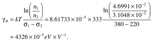
At the second step of FOAT, one can use, without conducting additional testing, the information from the first step, its duration, and outcome, and let the second step of testing has shown that after t₂ = 3bh of testing at the same temperature of Г = 60°С = ЗЗЗК, 98% of the tested samples failed, so that the predicted probability of nonfailure is P₂ = 0.02. If the stress o₂ is the elevated voltage c₂ = 220V, then the parameter n₂ becomes

and the sensitivity factor y_c for the applied stress is

The zero-stress activation energies calculated for these parameters n, and n₂, and the stresses o_: and a₂ is

To make sure that there was no calculation error, the zero-stress activation energy can also be found as

No wonder that these values are considerably lower than the activation energies of “healthy” products. Many manufacturers consider as a sort of “rule of thumb” that the level of 0.7eV can be used as an appropriate tentative number for the activation energy of healthy electronic products.

In this connection, it should be indicated that when the BIT process is monitored and the activation energy U₀ is being continuously calculated based on the number of the failed devices, the BIT process should be terminated, when the calculations, based on the observed and recorded FOAT data, indicate that the stress-free activation energy t/о starts to increase.

TABLE 11.3

TTF versus Probability-of-Nonfailure

The MTTF can be computed as

The TTF, however, depends on the probability of nonfailure. Its values calculated as TTF = MTTF x (In/⁵) are shown in Table 11.3.

Clearly, the probabilities of nonfailure for successful BITs should be low enough. It is clear also that the BIT process should be terminated when the calculated probabilities of nonfailure and the activation energy U₀ start rapidly increasing. Although our BIT analyses do not suggest any straightforward and complete way of how to optimize BIT, they nonetheless shed useful and insightful light on the significance of some important factors that affect the BIT’S need, and, if decided upon, its required time and stress level for a packaged product comprised of mass-produced components.