Basic Equations

Let an elongated bimaterial adhesively bonded or soldered assembly be manufactured at an elevated temperature then cooled down to a low (say, room) temperature and then, prior to ALT testing, subjected to mechanical compression applied to the assembly component with the lower coefficient of thermal expansion (contraction), as schematically shown in Figure 10.2. It is this component that will experience compressive thermal stress.

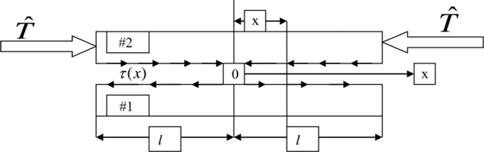
FIGURE 10.2 Birnaterial assembly subjected to the combined action of thermally induced and compressive external forces applied to the assembly component that will experience compressive thermal stresses during accelerated testing.

The longitudinal interfacial displacements щ(х) and u₂(x) in the assembly components #1 and #2 can be evaluated, in an approximate analysis, by the following formulas based on the concept of interfacial compliance:

where о.! and a₂ are the coefficients of thermal expansion (CTE) of the component materials, At is the change in temperature,

are the axial compliances of the components, £i and E₂ are Young’s moduli of the materials, V| and v₂ are their Poisson’s ratios, h and h₂ are the thicknesses of the components, T are the external “mechanical” compressive forces (per unite assembly width) acting on the low expansion component #1,

is the force acting in the cross section x of component #2, / is half the assembly length, т(л') is the interfacial shearing stress,

are the longitudinal interfacial compliances of the assembly components in the case of a long enough and/or stiff enough assembly,

are the shear moduli of the materials, and w,(x) and w₂(x) are the component deflections. The origin of coordinate x is in the mid-cross section of the assembly at the interface. The first terms in (10.15) are stress-free thermal contractions. The second terms are evaluated based on Hooke’s law assuming that the longitudinal displacements are the same for all the points of the given cross section. The third terms are “corrections” to this assumption and account for the fact that the interfacial longitudinal displacements are somewhat larger than the displacements of the inner points of the cross section. The fourth terms are due to bending.

The condition of the compatibility of the displacements (10.15) can be written as

where

is the longitudinal interfacial compliance of the bonding layer, h₀ is its thickness,

is the shear modulus of the bonding material, and E₀ and v₀ are its elastic constants. Introducing formulas (10.15) into condition (10.20), we obtain the following integral equation for the shearing stress function, x(x):

where Да = а₂ - a, is the difference in the CTE of the component materials, and

is the total longitudinal interfacial compliance of the assembly. As evident from equation (10.23), the “external” thermal strain ДаД? can be enhanced, without broadening the temperature range, by mechanical prestressing one of the assembly components. Equation (10.23) indicates also that such an enhancement increases with an increase in the axial compliance of the compressed component. From (10.23), we find by differentiation:

Treating the assembly components as elongated rectangular plates, we proceed from the following equations of bending (equilibrium):

where p(x) is the interfacial peeling stress (i.e., normal interfacial stress acting in the through-thickness direction of the assembly), and

are the flexural rigidities of the components. From (10.28), we find by differentiation

Solving equations (10.31) for the fourth derivatives of the deflection functions and substituting the obtained expressions into equation (10.27), we obtain the following equation:

that couples the interfacial shearing stress x(x) and the interfacial peeling stress p(x). In the obtained equation,

is the total axial compliance of the assembly (with consideration of the effect of bending), and

is the factor of the peeling stress. As evident from formula (10.33), the total axial compliance of the assembly increases with a decrease in the flexural rigidities of its components. As to the factor (10.34), it is the lowest for adherends with close flexural rigidities and is the highest in the case of considerably different rigidities.

We assume that the peeling stress is related to the deflections w,(x) and w₂(x) as

where К is the through-thickness stiffness of the assembly. Formula (10.35) reflects an assumption that no peeling stress could possibly occur in the given cross section, if the deflections w,(x) and w₂(x) are the same in this cross section. In an approximate analysis, by analogy with the longitudinal interfacial stiffness (compliance), one could assume

This formula indicates that while the entire bonding layer experiences stresses acting in the thorough-thickness direction of the assembly, only the inner portions of the assembly components, that is, the regions adjacent to the interface, are in the state of appreciable stress. From (10.35), we have

Solving equations (10.31) for the fourth derivatives of the deflection functions and substituting the obtained expressions into equation (10.37), we come up with another equation that couples the interfacial shearing, t(x), and the interfacial peeling, p(x), stresses

where

is the parameter of the interfacial peeling stress. Equation (10.38) indicates that the longitudinal gradient of the interfacial shearing stress plays the role of the external loading for the peeling stress: the greater this gradient, the higher is the peeling stress. It is noteworthy that equation (10.38) has the form of the equation of bending of a beam lying on a continuous elastic foundation. In the engineering theory of such beams, this equation is being written, however, for the deflection function, and not for the peeling stress.

Equations (10.32) and (10.38) are the two basic equations in the problem in question. These equations indicate that the two types of the interfacial stresses are coupled. Separating the functions x(x) and p(x) in equations (10.32) and (10.38), we find that these two functions could be determined, in effect, from the same equation:

or

Here,

is the parameter of the interfacial shearing stress. The solution to equation (10.40) should be sought, however, in an antisymmetric form and should contain only odd functions, while the solution to equation (10.41) should be symmetric with respect to the mid-cross section of the assembly and should contain therefore only even functions. This circumstance is reflected by the appropriate boundary conditions.

Boundary Conditions

Since there are no external forces acting at the ends of component #2, the force T(x) must be zero at the end x = l of this component:

Since no concentrated bending moments act at the assembly ends, the curvatures w"(x) and u'"(.v) must be zero at these ends:

As to the lateral forces, the following boundary conditions have to be fulfilled:

The first condition in (10.45) indicates that the lateral projection of the external force T should be equilibrated by the elastic force. Considering, however, that a typical electronic or photonic assembly is stiff enough, so that the angle of rotation w'(l) is small, and, in addition, that the external force T should be sufficiently low (actually, well below its critical value), one could assume, in an approximate analysis, that the third derivative w"'(l) of the deflection function for the component #1 can also be put equal to zero. Then, conditions (10.45) can be substituted, in an approximate analysis, with the following conditions:

The peeling stressp(x) must be self-equilibrated. This means that the following equilibrium conditions are to be fulfilled:

Equation (10.25), considering conditions (10.43) and (10.44), results in the following boundary condition for the shearing stress function:

Equation (10.26), considering (10.46), yields

Note that equation (10.28), considering the boundary conditions (10.44), (10.46), and the second condition in (10.47), is always fulfilled at the assembly ends.

Equation (10.30), taking into account conditions (10.46) and the first condition in (10.47), yields

Then, formula (10.49) also results in a zero-boundary condition for the second derivative of the shearing stress function:

As to the peeling stress, we obtain from (10.35), considering (10.44) and (10.46), the following conditions:

Solutions to the Basic Equations

We seek the interfacial shearing stress function x(x) in the form

By differentiation, we find

Then, equation (10.40) results in the following three equations for the factors Y1.Y2 and y:

where

is the parameter of coupling of the interfacial stresses. This parameter, as follows from formula (10.34), is very small if the assembly components have close flexural rigidities. Introducing new unknowns, % and q, as

we obtain equations (10.60) and (10.61) in the form

Introducing the q² value from equation (10.66) into equation (10.65), we obtain the following cubic equation for the unknown :

After the value is found, the q value can be determined from equation (10.66), and then the Yi and y₂ values could be evaluated as

These values are close to each other, if the £, value is small, and the q value is large. In such a case, as one could see from equation (10.66), q = 2p². Note that the result (10.68) could be obtained, if equation (10.41) and the particular solution

for the peeling stress p(x) were considered.

Constants of Integration

The constants C_b C₃, and C₅ of integration in the expression (10.53) for the interfacial shearing stress can be found, based on boundary conditions (10.58), (10.50), and (10.51) from the following system of equations:

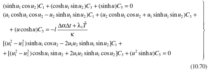
Here, the following notation is used:

As to the constants C₀, C₂, and C₄ in expression (10.69) for the interfacial peeling stress, p(x), they can be determined after substituting solutions (10.53) and (10.69) into equation (10.32) or into equation (10.38) and comparing the expressions at the left and the right parts of the obtained relationships. This leads to the following formulas for the constants C₀, C₂, and C₄ of integration:

Numerical Example

Input data

Component #1: Young’s modulus: E_{ = 12300 kg/mm²; Poisson’s ratio: V| =0.24; CTE: «i = 2.2 x 10^-6 1/°C; Thickness: 1ц = 0.5 mm; External force: T = 8.0 kg/mm;

Component #2: Young’s modulus: E₂ = 2000 kg/mm²; Poisson’s ratio: v₂ = 0.30; CTE: a₂ = 13.2xl0'⁶ 1/°C; Thickness: h₂ = 1.5 mm;

Bonding layer: Young’s modulus: £₀ = 200 kg/mm²; Poisson’s ratio: v₀ = 0.40; Thickness: /t₀ = 0.05 mm;

Change in temperature: At = 100°C; Assembly length: 21 = 20 mm

Computed data

Thermal strain: AaAt = (a₂-a_t)At = 11 x 10"⁶xlOO = 0.0011.

Axial compliances, as predicted by formulas (10.16):

Shear moduli, as predicted by formulas (10.22) and (10.19):

Interfacial shearing compliances, as predicted by formulas (10.21), (10.18), and (10.24):

Boundary condition for the interfacial shearing stress, as given by formula (10.48):

Note that because of the prestressing of the low expansion component of the assembly, the interfacial stresses in the assembly increase by a factor of 1.9. Flexural rigidities of the assembly components (treated as elongated rectangular plates) are evaluated on the basis of formulas (10.29):

Total axial compliance of the assembly, as predicted by formula (10.33):

Parameter of the interfacial shearing stress, as given by formula (10.42):

Factor of the peeling stress, as given by formula (10.34):

Through-thickness stiffness, as predicted by formula (10.36):

Parameter of the peeling stress, as predicted by formula (10.39):

Parameter of coupling of the interfacial stresses, as predicted by formula (10.63): Equation (10.67) for the unknown % value yields

and has the following root: 2, = 0.00615. Then, equation (10.66) yields q = 1.10047. From formula (10.68) we find

Note that the obtained two values are very close to each other and to the [) value. This is because the q value turned out to be substantially larger than the value, which is the case for adherends with not-very-much-different flexural rigidities. Equation (10.62) for the у value yields

Its root is у = 1.0165 mm⁴ and is not very much different from the к value.

The parameters щ = У/, u₂ = y₂/, and и = у/, expressed by formulas (10.71), are as follows:

These parameters are large enough, so that the assembly can be treated as an elongated one. Equations (10.70) for the constants C_b C₃, and C₅ of integration yield

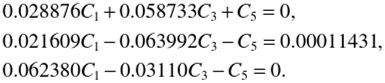
TABLE 10.2

Calculated Interfacial Shearing Stresses

These equations have the following solutions:

The shearing stress in the region close to the assembly ends can be computed by formula:

which can be obtained from solution (10.53). The calculated stresses are shown in Table 10.2:

At the bottom line, the stresses calculated using the simplified formula

are indicated. The calculated data indicate that this formula can be used for conservative engineering assessments. For the interfacial peeling stress, we obtain on the basis of solution (10.69),

The computed peeling stress is shown in Table 10.3. These data indicate that this stress is indeed self-equilibrated.

We conclude that the application of mechanical prestressing provides an effective means for achieving a failure-mode-shift-free “destructive ALT effect” in electronic and photonic devices. A simple and easy-to-use analytical predictive model has been

TABLE 10.3

Calculated Peeling Stresses

developed to assess the magnitude and the distribution of the interfacial shearing and peeling stresses in a bimaterial assembly subjected to the combined action of thermally induced and external (“mechanical”) loading during ALTs. A simplified predictive model developed earlier [11] can be used for conservative engineering assessment of the level of the induced interfacial shearing stress. The peeling stress should be evaluated, however, based on a more accurate model of the type suggested in [11] and modified in this paper. We would like to point out that our objective was not to come up with the most accurate predictions possible, but rather to obtain approximate, although still physically meaningful solutions, suitable for the application in engineering practice.

Note that our model has applications in prognostics and systems health management (PHM). This is a process of predicting the future reliability of the system by assessing the extent of deviation or degradation of a product from its expected normal operating conditions in a preemptive and opportunistic manner to the anticipation of failures. This can enable continuous, autonomous, real-time monitoring of the health conditions of a system by means of embedded or attached sensors with minimum manual intervention to evaluate its actual life-cycle conditions, to determine the advent of failure, and to mitigate system risks. The benefits of PHM include: (1) providing advance warning of failures; (2) minimizing unscheduled maintenance, extending maintenance cycles, and maintaining effectiveness through timely repair actions; (3) reducing the life-cycle cost of equipment by decreasing inspection costs, downtime, and inventory; and (4) improving qualification and assisting in the design and logistical support of fielded and future systems.