Data Reduction

Corrected Pressure-Volume Curve

The reduction of prebored PMT data involves the manipulation of the field data 1-min pressure and volume/diameter data to obtain a corrected cavity pressure vs. cavity volume or diameter/ radius curve by using the membrane and system calibrations as previously discussed. Use of the Menard rules for the design of foundation requires that specific parameters be obtained from

Figure 7.10 Idealized corrected PMT pressure-volume expansion curve.

the results of the test. Primarily, these parameters include: P_Q, P_f, P_L E_UR, and E_m, as defined in Figure 7.10. As can be seen, the PMT curve has three distinct zones: Zone 1 - pressure to inflate the membrane against the sides of the borehole and reinstate lateral stress from unloading by drilling; Zone 2 - pseudo-elastic straight-line pressure-volume response; and Zone 3 - plastic response after the pseudo-elastic response as the soil approaches a failure condition.

Initial Pressure, PО

The pressure P_Q is designated as the pressure that identifies the beginning of the elastic portion of the pressuremeter curve. Effectively, it is the point of tangency at the end of Zone 1. In many soils, this stress corresponds to the final point along the curve at which the ground stresses have been reinstated in the cavity and therefore closely represents the in situ total horizontal stress. Stresses up to this point represent reloading to account for borehole stress relief, and deformations represent recompression to account for disturbance and relaxations.

Since the value of P_Q coincides with the beginning of elastic behavior, it may be determined from the point of tangency with the elastic portion of the curve as shown in Figure 7.11. Note that it may be necessary to enhance or enlarge the initial portion of the curve to obtain an accurate determination of P_Q. Note also that a sufficient number of data points are required both at the beginning of the test, i.e., expanding against the borehole and reloading, and in the pseudo-elastic portion (Zone 2), in order to allow a sufficient accuracy in evaluating P_Q. The initial pressure may also be interpreted from the creep curve as will bediscussed..

Creep Pressure, Pf

At the end of the elastic portion of the test (Zone 2), the soil has reached an initial yielding point, which signifies the beginning of plastic failure. The pressure at which this change in behavior occurs is called the creep pressure, P_f. It is effectively the point of tangency of the pressuremeter curve where the linear pseudo-elastic behavior ends. The value of P_f may also be estimated from the creep curve as will be shown in Figure 7.14. Both methods should be used to provide some redundancy in the estimate of P_f. Figure 7.12 shows PMT data on an expanded scale used to determine the creep pressure.

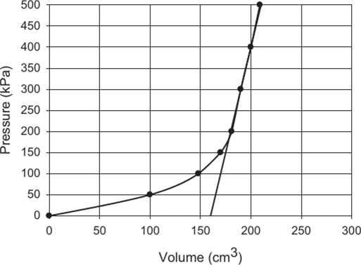
Figure 7.11 Identification of POT for initial pressure, P₀ = 200 kPa, using expanded scale.

Figure 7.12 Identification of POT for creep pressure, P_f = 550 kPa, using expanded scale.

Limit Pressure, PL

As pressure is increased above the initial yield point, an expanding annulus of plastic soil develops around the cylindrical cavity. When a cylindrical cavity is expanded in an elastic- perfectly plastic soil, the limit pressure P_L is theoretically reached when the infinite expansion of the cavity occurs, i.e., AV/V = 1. That is, the change in cavity volume is equal to the current cavity volume. Because of mechanical limitations, pressuremeters are not capable of expanding sufficiently to reach the limit pressure, and therefore, the estimation of P_L requires the extrapolation of data from lower values of AV/V.

In a prebored pressuremeter, the limit pressure is defined as the pressure where the probe volume reaches twice the original soil cavity, defined from volume measurements as V_D + V;. V, is the corrected volume reading at the pressure where P_Q is obtained, i.e., where the probe membrane made contact with the borehole wall. Therefore, the limit pressure, P_L, would be

Figure 7.13 ASTM method of extrapolating to obtain P_L.

obtained as the pressure where the volume is equal to 2 (V„ + V;). ASTM D4719 suggests that the limit pressure may be obtained by extrapolation to this volume by making a plot of 1/V vs. P, as shown in Figure 7.13. Only the data points obtained after the linear portion of the pressuremeter curve, i.e., after P„ should be used in this extrapolation.

Net Limit Pressure, PL*

The net limit pressure P*_L combines the extrapolated value of P_L and the interpreted value of P_Q as:

The net limit pressure is often used in design calculations for bearing capacity.

Pressuremeter Modulus, Em

The pressuremeter modulus may be determined using the slope of the pressure-volume curve in the pseudo-elastic (linear) portion of the corrected PMT curve. According to ASTM D4719, the pressuremeter modulus is determined from:

where

u = Poisson’s ratio

Vo = volume of the measuring portion of the uninflated (at rest) probe at 0 volume reading at the ground surface (cm³)

V = corrected volume reading of the measuring portion of the probe ДР = corrected pressure increase in the center part of the straight-line portion of the pressure-volume curve

AV = corrected volume increase in the center part of the straight-line portion of the pressure-volume curve corresponding to AP pressure increase V_M = corrected volume reading in the center portion of the AV volume increase Vo + V = current volume of inflated probe

If the diameter of the probe is measured during the test, the pressuremeter modulus may be determined from:

where

R_P = radius of probe in uninflated condition (mm)

AR_M = increase in radius of probe up to the point corresponding to the pressure where E_m is measured (mm)

dAR = increase in radius of the probe corresponding to AP pressure increase (mm)

AR = increase in probe radius (mm)

RP + AR = current radius of inflated probe (mm)

Unload-Reload Modulus, EUR

If an unload-reload loop is performed (recommended on most tests), Equations 7.2 or 7.3 may be used to determine the unload-reload modulus, E_UR. Briaud (2013) noted that the problem with the unload-reload modulus is that it is not necessarily a unique value for a given test. It depends on the amplitude of the unload-reload loop and also on the stress level where the unload-reload is performed. As a result, the value of E_UR may vary from operator to operator depending on the specific test procedures. Briaud (2013) recommended that the unload-reload loop be performed at the end of the pseudo-elastic part of the curve and that unload be taken to about Уг of the estimated pressure at this point.

Creep Curve

During the test, volume or diameter readings are taken at 30s and 1 min. after applying each pressure increment. The difference between these values is called the creep. In addition to plotting the full corrected pressure vs. volume/diameter curve, as shown in Figure 7.10, the creep curve is also plotted, as shown in Figure 7.14. Ideally, the creep volume will decrease as the pressure P_Q is approached, and then the pseudo-elastic portion of the curve will be very small and more or less constant up to the creep pressure, P_f, provided equal-pressure increments have been used in the test. After P_f, the creep volume will increase with each pressure increment as the limit pressure P_L is approached. The intersection of straight lines drawn through each section of the creep curve can also be used to interpret the initial horizontal stress, P_Q, and the creep pressure, P_f, as shown in Figure 7.14.

Figure 7.15 shows the results obtained using an NX-sized mono-cell PMT in medium stiff clay in Leona, Kansas. Even though the ASTM standard suggests obtaining the PMT curve in 7-10 pressure increments, the author has found that more data points, especially at the beginning of the test, are very useful in interpreting the value of P_Q, and it is essential to have at least 4-5 data points after the creep pressure P_f to accurately extrapolate the limit pressure P_L.

Figure 7.14 Idealized pressuremeter creep curve.

Figure 7.15 Test results obtained using a mono-cell PMT curve in Leona, Kansas.

Relationships Between PMT Parameters

Typical ranges in values of P*_L and E_m are given in Table 7.6 for both clay and sand. Even though the ranges are high in each category, it can easily be seen that clay values will generally be lower than sand values.

Results of the PMT may be used to give an indication of soil type based on the relationships between PMT parameters interpreted from the corrected PMT pressure-expansion curve. For example, Briaud (1992) suggested that clays show E_m/P*_L> 12 and sands show 7 < E_m/P*_L <12.

Similarly, according to Briaud (1992; 2013), in clays the P/P_L ratio is typically around 0.5, while for sands, it is around 0.33. Walker (1979) had shown that P(/P_L = 0.59 for the weathered rock at several sites in Canada and Australia. Bahar (1998) found that Pf/P_L = 0.56 for

Table 7.6 Typical range of expected values of P*_L and E_M

Figure 7.16 Observed relationship between P_fand P_L.

three stiff clay sites in Algiers. These interrelationships may be useful to check the quality of the test results but may also be used to make an approximate estimate of P_L in cases where the test does not give sufficient data points beyond the initial yield pressure.

Test results collected by the author from several published sources representing a large number of tests in a wide range of fine-grained soils are shown in Figure 7.16. Without any accounting for differences in test equipment or procedures and only considering the interpreted (or cited) values of P_f and P_L shows a very strong linear relationship over a wide range of stress. Results obtained by the author at eight test sites consisting of mostly finegrained soils are also shown. Figure 7.17 shows the same data as that of Figure 7.16 but on an expanded scale for lower values in softer materials. All of the data fall reasonably close to the trend line of P_L = 2 P_f.