Nonimaging Optical Systems

Limits to Concentration

The relationship between the concentration ratio and the angular field of view is a fundamental one that merits more than one demonstration. We shall give a thermodynamic argument in the context of solar energy concentration. Imagine the sun itself as a spherically symmetric source of radiant energy (Figure 4.1). The flux falls off as the inverse square of the distance R from the center, as follows from the conservation of power through successive spheres of area 4nR². Therefore, the flux on the earth’s surface, say, is smaller than the solar surface flux by a factor (r/R)², where r is the radius of the sun and R is the distance from the earth to the sun. By simple geometry, r/R=sin²# where в is the angular subtense (half angle) of the sun. If we accept the premise that no terrestrial device can boost the flux above its solar surface value (which would lead to a variety of perpetual motion machines), then the limit to concentration is just l/sin²0.

We call this limit the sine law of concentration. This relationship may seem similar to the well-known Abbe sine condition of optics, but the resemblance is only superficial. The Abbe condition applies to well-corrected optical systems and is the first order in the transverse dimensions of the image. There are no such limitations to the sine law of concentration, which is correct and rigorous for any size receiver. As already shown in Equations (2.14) and (2.15), there is an escape clause to this conclusion when the target is immersed in a medium with index of refraction (n) because then the limit is n²lsin#². Of course, the limit we have derived is for concentration in both transverse dimensions, which we will refer to as three-dimensional concentration (or 3D concentration for short). For concentration in one transverse dimension, which we will call two-dimensional (2D) concentration, the limit is clearly l/sind. While the concept of concentration in our demonstration refers to solar flux, implicit in our discussion is good energy throughput. We generally deal with concentrators that throw away as little energy as possible. Good energy conservation is an essential attribute of a useful concentrating optical system (see Figure 4.1).

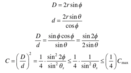
FIGURE 4.1 The flux from a spherically symmetric sun falls off ^ ^ j .

Imaging Devices and Their Limitations

If one were to ask the proverbial man on the street for a suggestion of how one might attain the highest possible level of concentration of, say, solar flux, a plausible response would be to use a good astronomical telescope—perhaps the 200-inch telescope on Mt. Palomar or any preferred telescope. Of course, such an experiment had better remain in the realm of imagination only, since beginner astronomers are would be admonished for pointing their telescopes at the sun at the risk of catastrophic damage to the instrument. But to continue this train of thought, the concentration limit of a telescope is readily shown to be ^S*ⁿ ^ after an elementary

4 sin' в

calculation (Figure 4.2). Here we have introduced a new parameter, ф, which is the rim angle of the telescope. The best one can do is make the numerator 1 for rim angle

f= 45°, so the best concentration achieved is —^— , which falls short of the fun-

4 sin^- в

damental limit by a factor of 4! Now factors of 4 are significant in technology (and

FIGURE 4.2 Image-forming solar concentrator for planar absorber.

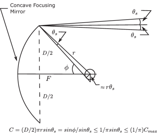
FIGURE 4.3 Image-forming solar concentrator for tubular absorber.

many other forms of human endeavor). It was the desire to bridge the gap between the levels of concentration achieved by common imaging devices and the sine law of concentration limit that motivated the invention of nonimaging optics. Entirely similar considerations can be applied to 2D or trough concentrators. A straightforward generalization to a strip absorber rather than a disk absorber gives a limit for, say, a

parabolic trough of , with a consequent upper limit of —5— for rim angle

2sin0 2sin0

ф=45°. This would be a useful configuration for a photovoltaic concentrator, with the strip consisting of solar cells. However, a more useful geometry for a parabolic trough thermal concentrator is a tubular receiver (Figure 4.3). In that case, the concentration relation becomes ^S*ⁿ^ , which attains its maximum value of —j— at a 90° rim angle. я sin 0 л sin в

This helps to explain why parabolic solar troughs tend to have large rim angles. In either case, we fall significantly short of the sine law of concentration limit, this time by a factor of 2 or л, depending on the configuration. As we shall see later, this factor of 2 or я makes the difference between the possibility and impossibility of fixed solar concentrators. The possibility of fixed concentrators opens up a broad vista of solar energy applications.

Nonimaging Concentrators

These simple examples of imaging systems and their attendant shortfalls in concentrating performance (we could have examined lenses and reached similar conclusions) suggest that the requirement that an optical concentrator form an image is unduly restrictive. After all, we are after transport of radiant energy. Imaging the sun may be useful in solar astronomy or in the study of sun spots, but it has no obvious advantage in solar energy conversion systems. Thus, even taking a more empirical optimization approach, it is plausible that relaxing the imaging requirement has the potential of improving concentrating performance; in other words, one would expect to be able to trade off one against the other. Approaching the subject this way does lead to incremental improvements over various classical imaging designs such as parabolic reflectors. Our approach in this book is to show methods that actually attain, or closely approach, the theoretical sine law limit to concentration while maintaining high throughput, methods that bear little resemblance to classical imaging approaches. An analogy with fluid dynamics may be useful to bring this point home. In fluid dynamics, as in optics, a useful representation is in “phase space.” Phase space has twice the dimensions of ordinary space and consists of both the positions and momenta of elements of the fluid. In optics, the momenta are the directions of light rays multiplied by the index of refraction of the medium. In optics, as in fluid dynamics, the volume in this phase space is conserved, a sort of incompressible fluid flowing in this space of twice the number of physical dimensions. Now consider an imaging problem taking the simplest example of points on a line. An imaging system is required to map those points on another line, called the image, without scrambling the points (Figure 4.4a)—that is, to focus the rays issuing from every object point into their corresponding image points. All the rays issuing from a point are represented by a vertical line in the phase space, and the system is required to faithfully map line onto line (Figure 4.4b). That may appear quite demanding, but it is precisely what an imaging system is asked to perform. But suppose we consider only the boundary or edge of all the rays. Then all we require is that the boundary be transported from the source to the target. The interior rays will come along (Figure 4.4c). They cannot “leak out” because were they to cross the boundary, they would first become the boundary, and it is the boundary that is being transported. To complete the analogy, the volume of the container of rays is unchanged in the process. This is the conservation of phase space volume. It is very much like transporting a container of an incompressible fluid—say, water. The fact that elements inside the container mix or the container itself is deformed is of no consequence. To carry the analogy a bit further, suppose one were faced with the task of transporting a vessel (the volume in phase space) filled with alphabet blocks spelling out a message. Then one would have to take care not to shake the container and thereby scramble the blocks. But if one merely needs to transport the blocks without regard to the message, the task is much easier. This is the key idea of nonimaging optics.

The Edge-Ray Principle or “String” Method

Figure 4.4c suggests the notion of transporting the boundary or edge of the container of rays in phase space. This leads to one of the most useful algorithms of nonimaging optics. We shall see that transporting the edges only, without regard for interior order, allows attainment of the sine law of concentration limit. To motivate the method we begin with the statement that all imaging optical design derives from Fermat’s principle. The optical path length between object and image points are the same for all rays (Figure 4.5a). When this same principle is applied to “strings” instead of rays,

FIGURE 4.4 Comparing imaging with nonimaging in the phase space representation, (a) The spatial representation of source and destination, L, is the direction cosine, (b) The phase space representation of imaging optics, (c) The phase space representation of nonimaging optics (edge-ray method).

it gives the edge-ray algorithm of nonimaging optical design (Figure 4.5b). First we must explain what strings are, which is best done by example. We will proceed to solve the problem of attaining the sine law limit of concentration for the simplest case: that of a flat absorber. Referring to Figure 4.6, we loop one end of a “string” to a “rod” tilted at angle в to the aperture AA and tie the other end to the edge of the exit aperture B'. Holding the length fixed, we trace out a reflector profile as the string moves from C to A. From simple geometry, the relation BB' =AA sin# immediately follows. This construction gives the 2D compound parabolic concentrator, or CPC. Rotating the profile about the axis of symmetry gives the 3D CPC with radius (a)

FIGURE 4.5 Fermat’s principle for rays and strings.

FIGURE 4.6 String construction for planar absorber.

FIGURE 4.7 String construction for tubular absorber.

at the entrance and (b) at the exit. The 2D CPC is an ideal concentrator—that is, it works perfectly for all rays within the acceptance angle q (in 2D geometry). As we will see, the 3D CPC is very close to ideal in 3D geometry. The flat absorber case is a natural candidate for rotating about the axis because the square of the ratio of diameters (sin 20) agrees with the maximum concentration. Other absorber shapes such as circular cross-sections (cylinders in 2D, spheres in 3D) do not have this correspondence because the area of the sphere is 4л7/², whereas the entrance aperture area is /га². Notice that we have kept the optical length of the string fixed. For media with varying index of refraction («), the physical length is multiplied by n. Of course, we have not demonstrated that this construction actually works. One admittedly tongue-in-cheek approach is to state that anything this “neat”—in other words, that satisfies the conservation laws in a natural way—has to work. Perhaps a more serious “proof” is to notice that the 2D CPC rejects all stray radiation and therefore must be ideal for conservation of phase space (Ries & Rabl, 1994; Winston, 1970). The string construction is very versatile and can be applied to any convex (or at least nonconcave) absorber. Figure 4.7 shows the string construction for a tubular absorber as would be appropriate for a solar thermal concentrator.

This time 2m=BB' sin0, where a is the radius of the cylindrical absorber (Winston & Hinterberger, 1975).