Focal Function
The above example shows that a reflector Re R may have supporting paraboloids which are not among paraboloids in the family defining R. In fact, for any reflector R e R it is possible to construct a paraboloid of revolution with any given axis у and focus О supporting to R. This is a consequence of the boundedness and closeness of R. The proof of this fact is nearly the same as in the example above. That is, if P(y) is not already supporting to R, rescale P(y) homothetically into Py) so that p(m) < py(m) Vm e S2, where p' is the radial function of Py). Then decrease the focal parameter py) until Py) is supporting to R. Because R is a closed bounded surface, the number p’ can always be uniquely determined.
Based on this property, applicable to any yeS2 and any reflector Re'R, it is always possible to define for any Re'R a function p(y), у e S2, such that each paraboloid P(y) with focus О and focal parameterp(y) is supporting to R. This function is called the focal function of reflector R. Note that p(y) >0 Vy e S2, since the origin О is strictly inside the convex body bounded by R.
Using the focal function, Conditions (8.10) and (8.11) can be restated as follows: for each у ef for which the inf г on the right of Equation (8.9) is achieved, that is, P(y) is supporting, we have

Therefore, for each у ef

Clearly, the equality in Equation (8.12) holds for any paraboloid supporting to R, including those with axes у e S2 f. Thus, if R e R and if p(m), m e S2 and p(y), у e S2 are the radial and focal functions of R. respectively, then
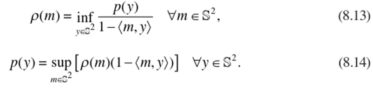
It can be shown that for any R e R the functions p, p e C(S2). The continuity of p is a consequence of convexity of R. Also, since R is bounded, the function p is bounded. The continuity of p follows from Equation (8.14) and the boundedness of p. Thus, with each reflector R e R we have a uniquely defined pair of continuous on S2 functions p, p> 0 satisfying Equations (8.13)—(8.14). Conversely, any pair of continuous and positive functions on S2 satisfying Equations (8.13)—(8.14) defines uniquely a reflector in R. Indeed, the family of paraboloids defined by p(y), у e S2, can be used as the family defining some R e 'ft in the construction (8.8). At the same time, by Equation (8.14) each paraboloid in this family is supporting to R. Clearly, such R is defined by p and p uniquely.
Note 8.4.1 It follows from the preceding considerations that, while we are dealing with the radial and focal functions defining a reflector Re R, we may assume that the sets D and T coincide with the sphere S2. However, as we will see in the following sections one has to deal carefully w'ith such assumptions if considerations involve the radiance and irradiance over the corresponding input and output apertures.
Generalized Reflector Map
Next, we want to extend the notion of reflector map to reflectors in 'R. In general, a reflector R eR may have points at which there is no tangent plane and the normal is not defined. Therefore, the reflected direction can not be defined using the reflection law (8.1). For example, in Figure 8.1 such points are A, B, and C. Note that at such a point there is more than one supporting paraboloid. Nevertheless, we can use Equation (8.9) to define an analogue of the reflector map, called the generalized reflector map.
Let R be an arbitrary reflector in R. For a point m e S2 the vector r(m)=p{m)m gives the corresponding point on R. It follows from Equation (8.9) that the inf is achieved for P(y) supporting to R at r(m). The image of m under the generalized reflector map—we denote it again by y(m)—is defined as

According to this formula, if at the point r(m) there is a unique supporting paraboloid then the unit vector in the direction of its axis is y(m). However, if at the point r(m) there is more than one supporting paraboloid then y(m) is the set of all unit vectors in S2 in directions of axes of the corresponding supporting paraboloids. Thus, in general, у is multivalued. It is also clear that the map g maps S2 onto T, as for each у e T there is a paraboloid with axis у supporting to R. If we include in our consideration all possible supporting paraboloids to R then clearly y(S2) = S2.
The points on a reflector R at which there is more than one supporting paraboloid are called singular. The nonsingular points are called smooth. Thus, a ray emitted from О in direction m e S2 is reflected off R at r(m) and produces a a set of directions y(m). If r(m) is a smooth point on R then g(m) consists just of one, uniquely defined, point. On the other hand, if r(m) is a singular point then this ray splits into a set of rays with directions y(m). This is consistent with the physical interpretation of diffraction. In this case, у is multivalued and, clearly, T a y(S2).
It turns out that the set of singular points on R is “small” in the sense explained later in Notes 5.1-5.2. Observe also that expanding the family of supporting paraboloids to R by including supporting paraboloids with axes of direction у e S2 T leaves the the radial function of R unchanged. It is also clear that a paraboloid defined by p(y) with у e S2 T can be supporting to R only at a singular point. Also, a supporting paraboloid P(y) is tangent to R at a smooth point only if у e T. It can be shown that any R e 'R is completely determined by supporting paraboloids tangent to R at smooth points; cf. Schneider (Schneider, 2014), Theorem 2.2.6.
Note that each tangent plane to a supporting paraboloid at the point of contact with R leaves the paraboloid and the reflector in one of the half-spaces defined by that plane; that is, this plane is supporting to R in the sense of convexity theory (Schneider, 2014). Thus, any singular point on R will also be singular in the sense of convexity theory, that is, at such a point the surface R has more than one supporting plane.
Note 8.5.1 Since reflectors in 'R. are convex surfaces, it is useful to recall some basic facts from convexity theory. These facts will often be used in this exposition. An extensive source for theory of convex surfaces is Schneider (2014). We also use here some basic notions of measure theory; see, for example, Lieb and Loss (1997) and Taylor (2006). Let R e TZ. On any convex surface it is possible to define Borel sets obtained from closed subsets of R by taking countable unions and intersections. Each Borel set on R has a well-defined (Lebesgue) measure (area) and we often refer to Borel sets on R as measurable. For a set A cz R we say that a property holds almost everywhere on A when it holds on AA where the measure of A’ is zero. It turns out that any reflector R e 'R is smooth almost everywhere. This follows from the fact that any tangent plane to a supporting paraboloid at the point of contact with R leaves the paraboloid and the reflector on one side defined by that plane. In convexity theory such planes are also called supporting. Thus, any singular point on R will also be singular in the sense of convexity theory because at such a point R has more than one supporting plane. By a known result in convexity theory the set of singular points on a convex surface has measure zero (Schneider, 2014, p. 89). Therefore, the set of singular points on a reflector in 'R also has measure zero.
Note 8.5.2 It is known from convexity theory that the set of points where a convex surface is not two times differentiable has measure zero (Schneider, 2014, p. 31). Thus, any R e R. is almost everywhere two times differentiable. From this we conclude, in particular, that the radial function defining a reflector is differentiable two times almost everywhere on S2. Furthermore, it was shown in Oliker (2002), on p. 160, that the focal function p of a reflector R e'R is also the support function of a closed, bounded convex surface in R3. By a known result in convexity theory (Schneider, 2014, p. 31), the focal function p is twice differentiable almost everywhere on R. The above observations imply also that for any R e R. the map у : S2 -> S2 is single-valued almost everywhere on S2.
Weak Solutions
In this section we work with input and output apertures D,f <= S2, respectively. Each of the apertures may coincide with the entire S2. The radiation /On), me D, of the source О is assumed to be nonnegative and integrable. Setting /(m)=0 for m in the complement of D in S2, we make / defined on the entire S2. In addition, / e L(S2). For a measurable set Г2 <= S2 the quantity
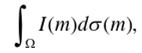
where do(m) is the surface area element of S2, is the total energy of the source emitted through the aperture Q.
In order to define the amount of energy transferred by reflector R from the source О to a subset coczf, we first need to introduce the inverse map y~' : T —> S2 which associates with each у ef the set of directions m of incident rays reflected by R in direction y. Analytically,

It was shown in Caffarelli and Oliker (2008) and, in more detail, in Oliker (2002) that for any measurable set со a T the set у-1 (со) is measurable on S2, and, therefore, the function

is a completely additive measure defined on all Borel subsets of f. Physically, G(R, со) is the quantitative expression of the amount of energy transferred by reflector R to the far-field region defined by reflected rays with directions ye со. Note that G(R, со) may not be absolutely continuous; that is, G(R, со) may be positive even if со consists of only one point.
Let function L define the required irradiance on T be as before, that is, L e L(T) and nonnegative. Extend L to the entire S2 by setting L(y)=0 when у e S2 T. Thus, LeL( S2).
Definition 8.6.1 A closed convex reflector Re 'R is called a weak solution to the FFR problem if

Equation (8.17) for the unknown reflector R together with Equation (8.16) is in terms of integrated intensities and it is called the weak form of the corresponding point- wise equation

which in turn is equivalent to Equation (8.3) if the latter is restated on T and treated as the target set under reflector map y. Evidently, for an arbitrary Re'R such a transition is not possible and Equation (8.17) is a physically motivated replacement of Equation (8.18).
Example 1. Here we provide a physical illustration of Equation (8.17) and its weak solution. Suppose T consists of only two points y1;y2,y, * y2 and

where <5(y-y,), /= 1,2 is the Dirac delta function on S2 concentrated at y,-. The reflector R is constructed using two paraboloids: P() with focal parameter p, and P(y2)) with focal parameter p2 » p. Assume that D is such that P() intercepts all light rays emitted by О through D. Then g(m)=y, for all m e D, det J(y(m)) = 0 everywhere in D, and y~‘(y,) = D. At the same time,

which is to say, all reflected light is concentrated at y,. Thus, Equation (8.17) is a physically correct description of this situation while the point-wise Equation (8.18) is not applicable.
Example 2. Suppose D = S2, T = {y1;y2}, у, ф y2,1 (in) = 1, and
i

Again, our reflector R is constructed with two paraboloids of revolution with axes y, and y2. Let p, and p2 be two positive numbers which we use as focal parameters of P(y,) and P(y2), respectively. It is clear that if p, and take p2 sufficiently large then for the corresponding reflector the area of the set g"1 (y2) will be small and consequently the integral

will have a small value; that is, the total irradiance from the source О reflected by R in direction y2 will be small. The analogous integral F(yl) will be nearly equal to F+F2. By decreasing p2 continuously we will obtain reflectors producing larger F(y2) and smaller F(y,). The required values of and F2 will be achieved at some value of p2. The corresponding pair of paraboloids combined as in Definition 3.1 is the weak solution to FFR in this case.
The following important property connects the energy G transferred by a reflector, the generalized reflector map y, and the input radiance I.
Theorem 8.6.2 For any reflector R e'R. and any continuous function h on S2 the following equality holds:

where у is the generalized reflector map ofR. The integral on the left is taken with respect to the measure G(R, w) defined in Equation (8.16).
Because g is multi-valued only on a subset of S2 which has zero area, the integral on the right of Equation (8.19) is well defined. The proof of this property is analogous to the proof of Lemma 4.9 in Glimm and Oliker (2004).

