Variational Approach
In the far-held problem the reflected directions are identified with points on the unit sphere S2. The target irradiance (often referred to as intensity or irrradiance intensity) in this case is the flux per unit area of the aperture on S2 representing the directions of reflected rays, W/sr; see Figure 7.1.
It follows from the discussion in the previous section that the numerical solution of the semi-discrete version of the FFR problem is the critical step. The variational formulation of the FFR problem in the weak form Equation (8.17) described later permits its reduction to a linear programming problem. Furthermore, the semi-discrete version upon a suitable discretization of the source radiance becomes a finite- dimensional linear programming (LP) problem whose solution is an approximation to the solution of the original problem. The LP setting for the FFR problem can be put in a form acceptable to available codes.
It is important to recognize that unlike the SQM the LP formulation is not possible in all optical design problems and in each case the required optimization problem must be formulated anew. In some cases, for example in near-field reflector/ refractor problems with one mirror/lens, a linear programming formulation is not available.
The organization of this section is as follows. First, in Section 9.1 we describe a special linear functional (9.5) and state a theorem establishing equivalence between solutions of (8.17) and maximizers of (9.5). In Section 9.2 we specialize the functional (9.5) to the semi-discrete case. In Section 9.3 we present a special discretization of the source radiance and formulate the corresponding LP problem. Finally, in Section 9.6 we present important general remarks indicating limitations on the applicability of the variational approach.
Everywhere in this section we continue to use the notations introduced in previous sections. The presentation here is a slightly modified version of presentations in our papers Oliker (2005) and Glimm and Oliker (2003).
The FFR Problem as an Optimization Problem
We continue to denote by D,T e= S2 two closed domains in S2 (the input and output apertures; see Fig. 7.1). As before, I(m) and L(y) are nonnegative integrable functions given on D and T, respectively, satisfying Equation (8.21), and extended to the entire S2 as zero in S2 D and S2 f, respectively. Again, m denotes a point in D and S2 D and у in T and S2 T. The set of closed convex reflectors as in Definition 3.1 is denoted, as before, by /7. We also use the same notation p to denote the extended focal function of R e 77.
For m, у e S2 put

It follows from (8.13)—(8.14) that any pair of functions p, p e C(S2) such that p, p > 0defines uniquely a reflector Re 11 if

and for each m there is a у and for each у there is an m such that
 The generalized reflector map у is defined as before in Equation (8.15):

Because p, p > 0 on S2, bounded, and K(m,y) = +
We formulate now the maximization problem associated w ith the FFR problem. First, we define the set of admissible pairs of functions:

Evidently, if p, p are the radial and focal functions of R e 'R then (log/?, log/?) is in Adm.(S2).
Let /, L be two functions as above. Consider the linear functional
 and the maximization problem

Clearly, T is continuous on C(S2)xC(S2) relative to the norm defined as max jmax„з I s l,max„2 I q l}.
Theorem 9.1.1 Let Re 'R and (p.p) e C(S2)xC(S2) be the corresponding radial and focal functions ofR. The following two statements are equivalent:
- (1) The pair (log/?, logp) is a solution of problem (9.6);
- (2) The reflector R=(p, p) is a weak solution of the FFR problem 8.17.
An immediate consequence of Theorem 9.1.1 is that the weak solution w'hose existence is guaranteed by Theorem 8.7.1 can be determined by finding a maximizer of functional T on Adm^(S2). The discrete version of this maximization problem can be solved by numerical methods of linear optimization; see Section 9.2. It can be shown that from the point of view of optimization the maximization problem (9.6) is the dual of the minimization problem which will be discussed in Section 9.3. In a slightly different form, Theorem 9.1.1 was proved in Glimm and Oliker (2003). The connection of the FFR problem with optimization was also independently shown in Wang (2004). Earlier, such connection for the two-mirror reflector problem was established in our paper Glimm and Oliker (2004).
Under an additional geometric assumption that D П T = 0 existence of a maximizer of T can be proved independently of Theorem 8.7.1; see the remark at the end of Section 5 in Glimm and Oliker (2003). It was shown in Gangbo and Oliker (2007) that this result holds under much weaker assumptions which allow the cost function (and their generalizations) to be infinite (Gangbo & Oliker, 2007).
Discrete Maximization Problem
In order to solve the maximization problem (9.6) numerically, we need to discretize the functional (9.5) and the constraints in Equation (9.4) and then solve the obtained discrete maximization problem. Below we describe this solution in detail.
Let M,N e N,M >l,N > 2, fix Appoints/и,,...,тм e S2 and N points у[,..., уN e S2 and in each case repeat the steps in Section 8.7.1. As a result we get M measurable subsets Cif* <= S2, i = 1,..., M, and N measurable subsets cof c= S2, j = 1,..., N, such that for each i = diameters Q-1 <3л / M and for each j = 1,...,N diameters
cof <Ъл IN, and for 1
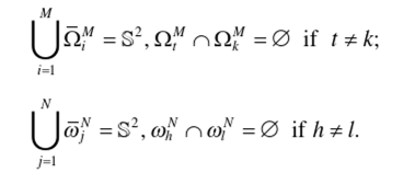
For i = 1,2,. . .,M and j = 1,2,...,N pick points m?1 e Clf and yf e Wj', and put

For measurable sets Q, со a S2 we define
 Assume that
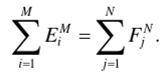
Put

and let

The maximization problem is to find = SM ,...,Su,qM = [qf ,...,qjH satisfying (9.7) and such that

Applying Theorem 9.1.1 (in its discretized version) we conclude that this problem is equivalent to the fully discrete problem obtained from the semi-discrete FFR problem (8.25) described in Section 8.7. Specifically, the required additional discretization is that of the apperture D (or S2), which has to be done anyway in problem (8.25) in order to compute G(R, со). Thus, the discrete FFR problem is now reduced to a solution of a discrete linear programming (LP) problem which can be done by known numerical methods (Rushendorf & Uckelmann, 2000); see also Merigot and Oudset (2016) for related results.
Connection with Optimal Mass Transport
According to the duality theory in optimization it is possible to construct a minimization problem dual to the maximization problem (9.6). By Theorem 9.1.1 this minimization problem must be related to the FFR problem. We describe now this connection following Section 4 of Glimm and Oliker (2003).
A variant of the celebrated Monge-Kantorovich optimal mass transport problem (Villani, 2009) in Euclidean space may be stated in our situation on S2 as follows. Let /C(m,y) be as in (9.1). Denote by V the set of maps P:S2 ->S2 which are “onto” and measure-preserving; that is, they satisfy the substitution rule

for all continuous functions h on S2. Each such map is called a plan. Note that a plan needs only be defined almost everywhere on sptl. Here,

where the overline indicates the closure of the set.
The Monge-Kantorovich mass transport problem we are interested in is: among all plans in V find a plan P minimizing the transportation cost

(The transportation cost may be infinite for certain plans; for example, the transportation cost is +00 if the plan is the identity map of S2 to itself.)
For weak solutions of the reflector problem the generalized reflector map is a plan by Equation (8.19). In fact, we have the following:
Theorem 9.3.1 Let R e 'R,, and p, p are the corresponding radial and focal functions of R. Suppose R is a solution of the FFR problem in weak form (8.17) and у its generalized reflector map. Then у minimizes the transportation cost (9.8) among all plans in V. and any other minimizer is equal to у almost everywhere on spt(I).
An important physical conclusion of this theorem is that the cost /C(m,y) encodes all the optical information needed for defining the required reflector. Theorem 3.1 can also be used to prove uniqueness of weak solutions to the FFR problem. The proof of this theorem is in Glimm and Oliker (2003); see Theorem 4.1.
Theorem 9.3.2 (see Glimm & Oliker, 2003) Let R. R' e 1Z be two weak solutions of the FFR problem with the same data. Let p, p' be their respective radial functions. Then R and R' differ only by a homothetic transformation; that is, there exists some c = const > 0 such that p(m) = cp'(m) for all m e S2.
Uniqueness was already discussed after Theorem 8.7.1. Theorem 9.3.2 provides an alternative proof based on coincidence of generalized reflector maps.
Computed Reflector for FFR Problem—Point Source
Here we provide details on the designed with the SQM reflector in Figure 7.2 solving a FFR problem. As before, S2 is a unit sphere centered at the origin of the Cartesian coordinate system in 3D space R3.
Point source. The input aperture Cl on S2, defined by the radiating point source at the center of S2 (see Figure 9.1), and its radiance intensity are:

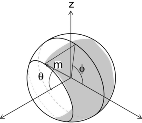
FIGURE 9.1 The shaded region on the unit sphere is the aperture C2 through which the light rays emitted by the point source at the center of the sphere travel into space; m is a unit vector in direction of such a ray.
The far-field Г and output intensity L are:
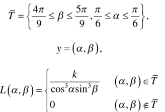
The output intensity L is chosen so that the designed reflector produces constant irradiance on a distant plane. The freeform reflector producing the required transformation has already been shown in Figure 7.2.
Note. Figures 9.1,9.2, and 9.3 are modified versions of figures from Benitez et al. (2006); reproduced with permission.

