The Flowline Method for Nonimaging Optical Designs
The Concept of the Flowline
We have seen that the edge-ray approach to nonimaging concentration has considerable flexibility in handling 2D problems. Its application in 3D is more limited, and, although useful designs are obtainable in 3D, these fall short of ideal concentration. This motivates the search for alternatives to edge-ray designs, especially in 3D applications (Winston & Welford, 1979a).
In the geometrical optics approximation, we describe the propagation of light rays as trajectories in a six-dimensional phase space (p, x), where the components of .v are the generalized coordinates (x1; x2, x3) and the components of p are the generalized momenta. These momenta give the optical path length when the light ray traverses length ds through a medium with an index of refraction n by the relation nds=ptdxt + p2dx2+р^хъ. For example, in cartesian coordinates (x, y, z) the components of p are just the optical-direction cosines.
It is useful to picture the propagation of the totality of light rays as if it were a fluid flow in this six-dimensional space. This flow is subject to conservation theorems that are essentially geometric and follow from the law of propagation of light rays. These are loosely referred to as Liouville’s theorem, but they are more properly called the integral invariants of Poincare. For our purpose, the most useful invariant is constructed out of a vector 7 , whose components are

Postulating as always a medium with no attenuation or radiation sources, the surface integral of J , f J ■ dA is invariant so that J has zero divergence. We shall call J
the geometrical vector flux and the direction of J the flowline. Quantities like J occur in radiative transfer where J dA is proportional to the net flux through the surface element dA and in photometry where 7, is proportional to the illumination on the x, у plane. This is most readily seen by rewriting

where 0V is the inclination of the elementary beam to the z axis.
Lines of Flow from Lambertian Radiators: 2D Examples
All Lambertian radiators that subtend the same solid angle at a point, in the strict sense that they are bounded by the same cone, give the same vector flux 7 at that point. This can be made clear by some simple examples (see Winston & Welford, 1979b).
Consider a strip AA in the x, у plane, of width 2 in the у direction, as in Figure 6.1. A simple calculation shows that 7 points along the bisector of the angle APA, and its magnitude is 7 = 2sin0, where the angle APA = 20. From elementary geometry the lines of flow are confocal hyperbolae with A and A as foci. Notice that the difference of distances from P to the foci |AP| -|A'P| is constant along a flowline from the property of hyperbolae. As a second example, Figure 6.2 shows a semi-infinite strip. It is easily seen that the flowlines are confocal parabolas, with the focus at the end A of the strip. A final example is a wedge: Figure 6.3 shows an example where the wedge angle is 60°. In regions where only one face of the wedge is seen, the pattern is the same as for the semi-infinite strip of Figure 6.2. From any point where both faces are seen, the effect is of a uniform Lambertian source subtending an angle of 60°. Thus |7| is constant in this region, and the lines of flow- are parallel as indicated.

FIGURE 6.1 Lines of flow and loci of constant |j| for the two-dimensional strip: the width is taken as two units. The axes of circles are labeled with the values of |j|. The two sets of lines are not orthogonal because 7 is not derived from a scalar potential.

FIGURE 6.2 Lines of flow and loci of constant у for a semi-infinite strip.
Figure 6.4 shows a truncated 60° wedge RQQ'R', which is infinitely extended back from the apex with an included angle 20=60°. We have to consider four different regions in calculating vector flux fields; these are separated by the boundary lines of the wedge produced, as shown in broken lines, and they are labeled regions A (and А'), В, C (and C'), and D. A point P in region A receives flux only from the face RQ so that the |J| distribution is the same as for a semi-infinite strip; that is, the flowlines are confocal parabolas with focus at Q, and the loci of constant |J| are straight lines radiating from Q. If P is in region B, it receives flux only from the strip QQ', and again we have the result that the lines of flow are confocal hyperbolas with Q and Q' as foci, and the loci of constant |7| are arcs of circles through QQ and Q'. If
P is anywhere in region D, the source has the constant angular subtense 20; thus |j is constant at 2 sin 0 throughout this region, and the lines of flow are straight lines perpendicular to QQ'. Finally, in region C, point P receives radiation from RQ and QQ', and the angular subtend is 20 as shown in Figure 6.14. The direction of J thus bisects the angle between a constant direction (parallel to QR) and the radius from a fixed point Q' thus, the lines of flow in region C are confocal parabolas with focus at

FIGURE 6.3 Lines of flow and loci of constant |y| for a wedge.
Q' and axis through Q' and parallel to RQ. The loci of constant |J| are straight lines radiating from Q', since the angle 20 as constructed is constant along these lines. The lines of flow for a truncated wedge are shown in Figure 6.5. Recent advancement of flow line has shown that the flow lines within the ideal nonimaging concentrators the also form ideal nonimaging concentrators (Jiang 2016a, 2016b).

FIGURE 6.4 A truncated wedge of angle 20. The truncated QQ' is shown as forming equal angles with the two sides of the wedge, but in fact the argument is still valid if this is not so.

FIGURE 6.5 Lines of flow of J and labeled loci of constant |yj for the truncated wedge; only the loci below the line of symmetry are shown. The wedge angle is 60°.
D Example
A disk as a Lambertian radiator—that is, the circular opening of a blackbody cavity—is the most important example to consider. The components of J can be calculated by integrating expressions such as Equation (1.1) over the surface of the disk.
These integrations have been carried out for radiative transfer purposes, and we shall simply quote the results. Sparrow' and Cess (1978), for example, provide the details, and they also give a useful transformation of the surface integral over the disk into a line integral around its edge; this considerably simplifies the calculation.
Let c be the radius of the disk and take the coordinate axes as in Figure 6.6.
Then the components of J in the y, z plane, which from symmetry are all that need be considered, are given by
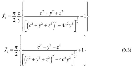
The slope of the lines of flow is given by arctan (JJJ.) and when this is calculated, it turns out that the lines of flow are the same hyperbolas as for the 2D case. The lines of flow in three dimensions are obtained by rotation about the z axis, as shown in Figure 6.7.
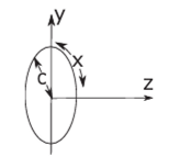
FIGURE 6.6 Geometry for calculating у for a luminous disk. Notice here x represents the radial direction instead of the Cartesian coordinates.

FIGURE 6.7 Lines of flow and loci of constant fl for a luminous disk.
A Simplified Method for Calculating Lines of Flow
In certain cases it is easier to calculate the etendue than to perform the preceding integrals. In cases where the etendue is known, we can use the solenoidal property of J to find the lines of flow. For example, in the case described by Figure 6.8, the etendue H from F, F' to A, A' is equal to [A'F]-[A'F'] in the 2D case and
»={[ЛТ]-[ЛТ-]}’/4 in the 3D case (the Hottel strings!) Then holding /^constant means we intercept a constant flux of J and therefore move along a line of flow. But holding the difference of distances to two foci, F, F'constant is the geometric definition of a hyperbola. Hence we recover the hyperbolic flowlines with lighter computation.
Assuming that there is a vector potential for J , V x A = J , and due to the axi- symmetric configuration of the problem, we can assume that only the x direction has nonzero value A,. Therefore the etendue H can also be represented by Н=2лАх. Because J. = (l / y)(5(yAv)/5y), Jy =-ЭА, /dz , we can also obtain the compo-
_ _ j / Л
nents of J due to its being the curl of A . Thus, the relations J, =- — and
1 ( 8H Л к >
J., =--- give Equation (6.3).
* 2 ay{dz)
Properties of the Lines of Flow
Let SL be a small surface element with a 100% reflecting mirror surface on one side. If we place <51 in a vector flux distribution at a point P (Figure 6.9) so the lines of flow lie in its surface, then the lines of flow locally on the mirror side will be undisturbed. To see this, we note that before the mirror is placed at position P, the resolved part of J normal to the surface is zero, since J lies along the lines of flow. Now this zero normal component is made up of equal and opposite components J* and Jn = -J* from rays coming from either side of S’L. But the effect of inserting the

FIGURE 6.8 Etendue for a luminous disk.
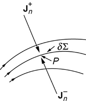
FIGURE 6.9 Placing a mirror in a vector flux field.
mirror is to remove Jn and replace it by J*, with reversed sign, according to the law of reflection, so there is no local disturbance.
The insertion of a mirror can, of course, disturb the lines of flow at some distance because it does not follow from Jn = -J*, that each ray from one side is paired witli a ray in the same plane of incidence and with the same angle of incidence on the other side. However, this simple situation does hold for a 2D vector flux field illuminated by a Lambertian radiator without obstructions and in the important case of a 3D field produced by a Lambertian disk.

