Appendix B: The Luneburg Lens
The Luneburg Lens
The Luneburg lens, discussed in Chapter 3, is not, of course, of any use as a practical concentrator. It is, however, the simplest example of an ideal concentrator with maximum theoretical concentration for collecting angles up to nl2, and therefore we develop its theory and general properties in this appendix. The main reference is to Luneburg’s own work (Luneburg, 1964). Some of the general geometrical optics background can also be found in Born and Wolf (1975), and extensions are given by Morgan (1958) and Cornbleet (1976).
Our starting point is the differential equation of the light rays. Let s be the distance along a ray measured from some fixed origin, let r be the position vector of a point on a ray, and let n(r) be the refractive index, varying continuously as a function of r. Then it can easily be shown (e.g., Born & Wolf, 1975, Section 3.2.1) that the rays are given by solutions of

Let the refractive index distribution have spherical symmetry. Then we can write n(r) = n(r), where r is a radial coordinate from the origin. Also, on account of the spherical symmetry, any light ray lies wholly in a plane through the origin, and we can describe its path by the polar coordinates (r,0).
In order to do this we note that dr/ds is a unit vector along the tangent to the ray—say, s. Now we have

from Equation (B.l). But by spherical symmetry grad n is parallel to rand so we have
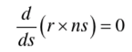 and a first integral of Equation (B.l) is
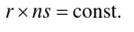
This is a vectorial equation that is equivalent to establishing the conservation of the skew relative to two orthogonal axes.
Since the rays are plane curves as just noted, this gives, say,

where ф is as in Figure B.l. Since

FIGURE B.1 Notation for ray paths in a medium with spherical symmetry.
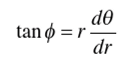
Equation (C.2) yields

and thus if n(r) is specified, the ray paths are obtained by quadrature

If we wish to find an index distribution n(r) that will act as an aberration-free medium, we have to regard Equation (B.4) as an integral equation for the function n(r). Luneburg did this and considered the use of an index distribution inside the unit sphere and with index unity at the surface of the sphere. He formulated the conditions for focusing from any point r0 to another r, as in Figure B.2, and he obtained an explicit solution for the case of present interest, r0 = oo, r, = 1.
Luneburg’s derivation is very complex and closely argued. Rather than reproduce his work we shall simply verify the solution he gave.
Let the lens have radius a and let the index vary in such a way that r has only one minimum value for the ray path in the lens—say, r*—as in Figure B.3. Then

FIGURE B.2 Luneburg’s general problem of an aberration-less unit sphere.
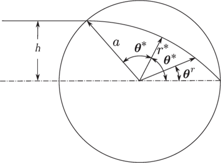
FIGURE B.3 Luneburg’s problem for r0=oo, t = 1.
from Equation (C.2) we have, using values at the beginning of the trajectory in the lens,
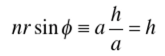
and thus

Since the two halves of the trajectory on either side of the radius r* must be mirror images we have

and thus Equation (C.4) takes the form

to be satisfied by a function n(r) for any h
Luneburg gave the distribution

as the solution of this integral equation. If we substitute for n(r), we have to evaluate

to verify the solution. From Equation (C.5) we find
 and if we make the change of variable
 in the integral, it becomes
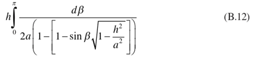
The indefinite integral has the value

and on substituting the limits of integration and recalling that h/a=sin 20*, we find that the value is 0*, as required by Equation (C.7). We have also obtained the actual ray paths, since these are specified by 0 as a function of r for given h by
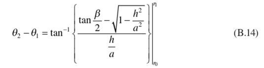
i
{ 2 Wf i 2
г h “
With sin /5 = 1 - — 1 —- . Figure B.4 shows several rays plotted to scale
L U'JjV a)
as in Figure B.5. A ray incident at height h from the center emerges at an angle to the surface arcsin(h/a) so that at any point on the exit surface rays emerge in all directions up to nil from the normal and the sines of the angles are distributed uniformly. Thus, the exit surface is filled with rays at all possible angles, and this must be in some sense a system with maximum theoretical concentration ratio. We can make this more explicit by calculating the entering etendue. This is, from Figure B.5, the area m2 sec 0 integrated over the direction cosines of the incoming beam—that is, it is

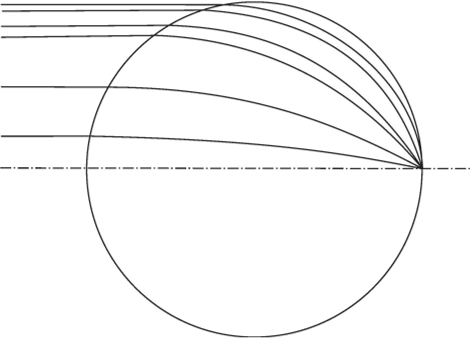
FIGURE В.4 Rays in the Luneburg lens.

FIGURE B.5 The Luneburg lens as a concentrator of maximum theoretical concentration ratio for any entry angle 0, less than n!4.
where ф is an azimuthal angle. The value of this is 2лга2 (l-cos0,). Also, the integral over the direction cosines alone is

and this is л sin2 в,. Thus the effective entry area must be л a1 / cos2 (1 /2)0,.
The area of the spherical cap that forms the exit surface is Ала1 sin2 (l / 2)0/ so that the concentration ratio is l/sin20/, the theoretical value for a collecting angle (),. Since all entering rays emerge, we have a 3D concentrator with the maximum theoretical concentration ratio.
We had to proceed in this slightly oblique way because the collecting aperture of the lens shifts with angle and because the exit surface is not planar. Thus, the correspondence with systems with well-defined and plane entry and exit apertures is not perfect.
References
Born, M., and Wolf, E. (1975). Principles of Optics, 5th Ed. Pergamon, Oxford.
Cornbleet, S. (1976). Microwave Optics. Academic Press, New York.
Luneberg, R. K. (1964). Mathematical Theory of Optics. University of California Press, Berkeley. CA.
Morgan, S. P. (1958). General solution of the Luneburg lens problem. ./. Appl. Phys. 29, 1358-1368.
Appendix C: The Geometry of the Basic Compound Parabolic Concentrator
The Geometry of the Basic Compound Parabolic Concentrator
It is probably simple to obtain the basic properties of the CPC from the equation of the parabola in polar coordinates. Figure C.l shows the coordinate system. The focal length/is the distance AF from the vertex to the focus. The equation of the parabola is, then,

This result is given in elementary texts on coordinate geometry, and it may be verified by transforming to polars the more familiar cartesian form of z. = y2/4/with axes as indicated in the figure.
We apply this to the design of the CPC as in Figure C.l. We first draw the entrance and exit apertures PP'and QQ' with the desired ratio in aperture between them, and we choose the distance between them so that an extreme ray PQ' (or P'Q) makes the maximum collecting angle 0, with the concentrator axis. Then according to Section
4.6 the profile of the CPC between P' and Q' is a parabola with axis parallel to PQ' and with focus at Q, and this parabola can be expressed in terms of the polar coordinates (r,
For the exit aperture we have, using Equation (D.l),
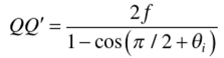
so that, if QQ' = la', in our usual notation
 Next we find

or

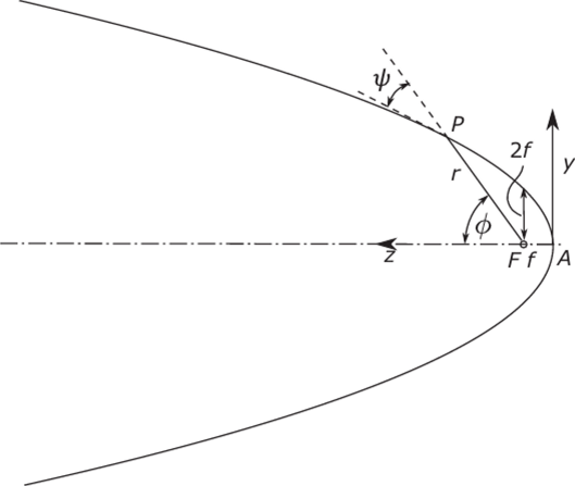
FIGURE C.1 The parabola in polar coordinates with origin at the focus, r = 2//(l- cosф) = f /sin2(1/2)0 .
Thus,

so that a = a' I sin ft, as required. Finally, for the length of the concentrator

This, of course, is again as required by the way we set up the design of the CPC.
It is obvious from the geometry of the initial requirements for the CPC that the profile at P and P' should have its tangent parallel to the axis. This also can be verified from the preceding formulation. For the tangent of the angle between the curve and the radius vector is, in polars,
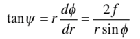
for the parabola, and if we put r = QP' and ф = 2ft, we find
 as expected.
The parametric representation of the CPC profile given in Section 4.6 is easily obtained from Figure C.2 if we take an origin for cartesian coordinates at the

FIGURE C.2 Design of the CPC.
center of the exit aperture and z-axis along the concentrator axis. We have from the figure

Appendix D: The θi/θo Concentrator
The 0/0o Concentrator
Figure D.l shows the concentrator with appropriate notation. From the triangle QQ'S we have

Also, since the angle RQS is к -Q„ - в,-, the triangle RQS is isosceles, and so QR = QS.
From the polar equation of the parabola,

so from Equation (D.l) we find for the focal length of the parabola

Again, using the polar equation of the parabola,
 and

From Equation (D.4) we find immediately

so that the 0/0,, concentrator is actually ideal in two dimensions.
The overall length of the concentrator is, from the figure,

just as for the basic CPC (Equation (D.4)).
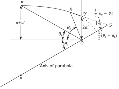
FIGURE D.1 Design of the в/в„ concentrator.
Appendix E: The Truncated Compound Parabolic Concentrator
The Truncated Compound Parabolic Concentrator
In this appendix we give the derivations of the formulas in Section 5.7. We show in Figure E.l the parabolic section in polar coordinates. For these coordinates we recall (see Appendix D) that the equation of the parabola is

If s is the arc length of the parabola, then
 so that

or

from Equation (E.l). We have to integrate this to find the arc length, which is proportional to the reflector area in a 2D system. We have to evaluate the indefinite integral

On making the change of variable
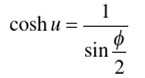
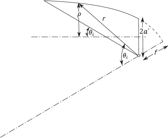
FIGURE E.1 Construction for the truncated CPC. we obtain
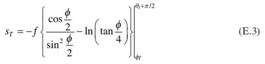
The radius of the entrance aperture is simply

which gives Equation (5.18) immediately. Thus, Equation (5.22) for s,tar is obtained. Likewise the length Lr of the truncated CPC is

from which Equation (5.19) follows immediately, and thence Equation (5.21).
For the 3D CPC the element of area of reflector is
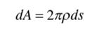
where p is the radius of the CPC at the current point. Since p is rsin(

This can be integrated by making the same change of variable, cosh и = cosec (012), and the result for the ratio of area of collection surface divided by area of collecting aperture is


