Near-Field and Far-Field Limits
It is useful to examine the pinhole radiometer and the formalism we have presented in two limiting cases. First, however, we explain some notation regarding the correlation operator and function (see Littlejohn and Winston, 1995, for more
details). The mutual coherence is defined by T(r,r') = t// (r )t// (r), where the overbar means a statistical or ensemble average, and where we use a scalar model for the wave field 4/, which in electromagnetic applications can be loosely identified with one of the components of the electric field. When z=z' we can associate the
mutual coherence with an operator IT(z) by r(F±,z;r±,z) = ^Fx|f (z)|/i^ , so that f(z) = |v/(z)<>V'(z)|-Thus,

Thus, if we identify |i//|~ with 4л times the energy density, then for paraxial rays (c/47r)Trf(z) is the power crossing the plane z,-
Now let us consider the case that a uniform, thermal source is very close to the radiometer, which is useful for normalizing the signal. Then at the entrance aperture the mutual intensity is proportional to a delta function, Г(г,г') = /Д2<5(г|_-г[), where I0 is a constant witli dimensions of energy/vol. A thermal source is not really delta-correlated, of course; the spatial correlation is really a sine function with a width of the order of a wavelength. It is for this reason that we insert the factor of 12 into the formula for the mutual coherence, so that if we need to set r± = r± for the purposes of taking the trace, we can interpret ЯЩ0) as being of order unity. In any case, when we compute the signal according to Equation (10.2), we obtain

where we set

for the number of phase space cells in the acceptance region of the instrument.
The trace of M is easy to compute. We first make the paraxial approximation in Equation (10.6), which gives

where the r" integration is taken over a circle of radius b. Now setting T = r[ and integrating T over a circle of radius a, we obtain

where d0 = b/L.
The number M has a simple interpretation. A phase space cell in the four-dimensional kL -rL phase space has volume (2л-)2. As viewed from the standpoint of the exit aperture b of the radiometer, the rays passing through each point of the aperture
( а V _ ( ka f
b occupy a solid angle of л- — , or a region of к-space of area n — . The region
) v L, ,
of r -space is just the exit aperture of area nb1. Multiplying these areas and dividing by (2л-)2 gives precisely TV,.
Next we consider the case of a very distant thermal source, which effectively produces a coherent plane wave at the entrance aperture, say, e'kz, so that
r± |f (z)|/± = /о (n6s)'. The dimensionless factor л0д2 will be explained below. Using this and Equation (10.10), we obtain

It is easiest to do the r± and r[ integrals first (both of which go out to radius a). These are identical, and are given by

where s = r± or r{. This leaves only the r[ integration (taken out to radius b)
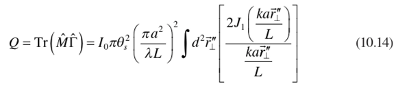
which agrees with the expected fraction of the Airy diffraction pattern contained by the detector of radius b.
A Wave Description of Measurement
We begin with the statistical properties of the incident wave field. The two-point correlation function at the source plane is

with r± and r[ inside the source, a, and equal to 0 otherwise. The matrix elements of the Fresnel free space propagator of a distance L are given by

where к=2л/А. The two-point correlation at a plane a distance L from the source in the Fresnel diffraction regime is

In Equation (10.17), Fr (rx -rx) is the Fourier transform of the source area; it is the VCZ result for the far-field two-point correlation function.
We will be testing two source geometries, circular and square. For the square geometry Fr is

with d the linear dimension of the source. For the circular geometry Fr is
Focusing and the Instrument Operator
The matrix elements for the lens operator are given by

The instrument operator is

where P is the propagator from the aperture, A(a), to the detector A(b).

The matrix elements for A (a) are given by

with F, and r± inside the aperture, a, and equal to 0 otherwise. The matrix elements for A{b) are given by

with Fl and r[ inside the detector, b, and equal to 0 otherwise.
From Equations (10.16) and (10.20) we have

This gives

with T inside the detector, r[ inside the aperture, and equal to 0 otherwise.
The matrix elements of M are given by

The integration is over the detector area.
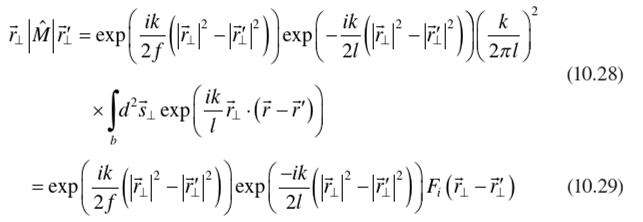
with r± and r[ inside the aperture, a, and equal to 0 otherwise. Here F, is
 If the camera is focused on the source

where L is the distance between the camera entrance aperture and the source. In this case the nonzero matrix elements are given by

The VCZ result for the nonzero matrix elements of M are given by Equation (10.30) with the camera focused at infinity, /=/ This results in a slight difference between the VCZ result and the general result in time phase space volume of M defined by

with Nj being time number of phase space cells. The infrared camera we used in the experiment has a circular entrance aperture and a square detector. We thus have

with rL and r[ inside the circular entrance aperture of radius a and equal to zero otherwise. The linear dimension of the square detector is 2b. From Equation (10.32),

where 20i=2b/l is the full acceptance angle. For all practical purposes, the difference in the values of V, for the focused case and with /=/is negligible. Henceforth, we will mean /=/when referring to Nr
Measurement by Focusing the Camera on the Source
From Equations (10.17) and (10.32), the detected signal, Q, is
 The normalized signal, Q„, is defined as

Experimental Test of Focusing
The matrix elements of the instrument operator modeling the infrared camera used in the experiment are given by Equation (10.32). The experiment was conducted by focusing the camera on the source. The results of the experiments are compared with Equations (10.36) and (10.37).
The following is the protocol for processing the data. The value of the signal when the detector of the camera is flood-illuminated by the blackbody radiation subtracted by the value of the signal when the detector is flood-illuminated by the background is used as the normalization. The measured normalized signal is obtained by first subtracting the detected signal from the background and then dividing by the normalization. The normalized signal is compared with theory.
The camera has an interference filter and a HgCdTd detector giving a wavelength window with a peak at 2 = 8.8 mm and Д2=±0.75 mm. The square HgCdTd detector is of dimensions 75 mmx75 mm. The focal length of the camera is/= 18.99 mm. In Equation (10.32) Fi is then given by Equation (10.30), with /> = (75/2) pm.
Two circular aperture plates of radii « = (). 136in and « = 0.272in were placed in front of the camera aperture. We have N~ 1.888 for the a=0.136 in aperture and N,=7.551 for the a=0.212 in aperture. The face of each plate facing the lens was painted with high emissive paint to provide the background. Time, source, size, and shape were controlled by placing aluminum masks with either square or circular apertures over a blackbody source set at T ~ 500°C.
Define Nr as

where the integration is over the camera aperture. Nr can be interpreted as the number of phase space cells of the radiation field intercepted by the camera aperture. Therefore, Nr can be much less than one without violating the uncertainty principle. For a square source

and for a circular source

Here 0S is the half angle subtended by the source at the camera’s entrance aperture. For the square source 6s=d/2L with d being the linear dimension for the square source. For the circular source 0s=d/2L with d being the diameter of the circular source.
The results of the measured normalized signal are plotted with theory versus Nr in Figures 10.4 and 10.5. The agreement with the experiment is highly satisfactory.
Conclusion
We have demonstrated a consistent approach to incorporating the diffraction properties of the instrument in optical measurements. We used a remarkable analogy between the result of measuring radiance and the van Cittert-Zernike theorem that exploits the symmetry between an incoherent source whose radiance is being measured and the detector whose signal represents the measurement. It turns out that the measured radiance is represented (up to an overall constant) by the double integral over time instrument aperture of the mutual intensity of the field and the mutual
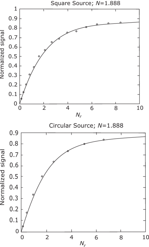
FIGURE 10.4 Comparison of experiment with theory for the N= 1.888 peak measurements. Filled circles are data points.
intensity of a delta-correlated source the same size, shape, and location as the detector. While we have expressed our results in a time context of radiometry, one would go through a similar analysis in analyzing the detection of any partially coherent wave. The signal is represented by the double integral of two mutual coherence functions. One of these is for the incident wave, the other arising from the detector considered as a source. It is likely that entirely similar considerations may apply to other signal detection processes where diffraction effects are important.
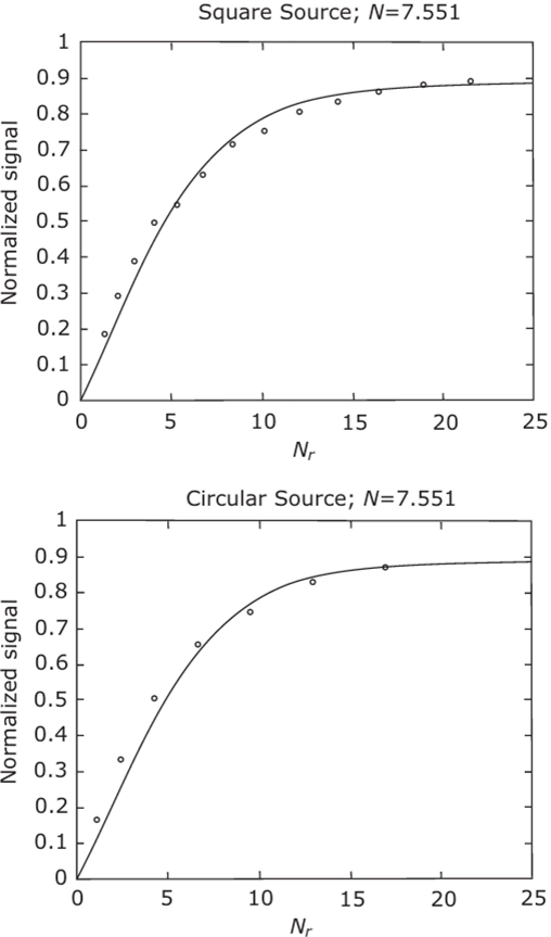
FIGURE 10.5 Comparison of experiment with theory for the A'=7.551 peak measurements. Filled circles are data points.
References
Born, M., and Wolf, E. (1999). Principles of Optics, 7th Ed. Cambridge University Press. Littlejohn, R. G., and Winston, R. (1993). Corrections to classical radiometry../. Opt. Soc. Am. A 10, 2024-2037.
Littlejohn, R. G., and Winston, R. (1995). Generalized radiance and measurement. J. Opt. Soc. Am. A 12. 2736-2743.
Mandel, L., and Wolf, E. (1995). Optical Coherence and Quantum Optics. Cambridge University Press.
Mather, J. C., Toral, M., and Hemmati, H. (1986). Heat trap with flare as multi-mode antenna. Appl. Opt. 25. 2826-2830.
Sun, Y., Winston, R., O’Gallagher, J. J., and Snail, K. A. (2002). Statistical optics and radiance measurement in the diffraction limit. Opt. Commun. 206, 243-251.
Walther, A. (1973). Radiometry and coherence.J. Opt. Soc. Am. A 63, 1622-1623.
Winston, R., and Littlejohn, R. G. (1997). Measuring the instrument function of radiometers. J. Opt. Soc. Am. A 14. 3099-3101.
Winston, R., Sun, Y., and Littlejohn, R. G. (2002). Measuring radiance and the van Cittert- Zernike theorem. Opt. Commun. 207,41-48.
Wolf, E. (1978). Coherence and radiometry. J. Opt. Soc. Am. A 68, 6-17.

