Light Cones

A primitive form of nonimaging concentrator, the light cone, has been used for many years (see, e.g., Holter et al., 1962). Figure 4.8 shows the principle. If the cone has semiangle у and if ft is the extreme input angle, then the ray indicated will just

( 6

pass after one reflection if 2y = — - ft. It is easy to arrive at an expression for

V 2 )

the length of the cone for a given entry aperture diameter. Also, it is easy to see that some other rays incident at angle ft, such as that indicated by the double arrow,

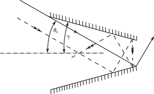
FIGURE 4.8 The cone concentrator.

will be turned back by the cone. If we use a longer cone with more reflections, we still find some rays at angle 6_j being turned back. Clearly, the cone is far from being an ideal concentrator. Williamson (1952) and Witte (1965) attempted some analysis of the cone concentrator but both restricted this treatment to meridian rays. This unfortunately gives a very optimistic estimate of the concentration. Nevertheless, the cone is very simple compared to the image-forming concentrators described in Chapter 3 and its general form suggests a new direction in which to look for better concentrators.

The Compound Parabolic Concentrator

The flat absorber case occupies a special place because of its simplicity. Historically it was the first to be discovered. For these reasons its description and properties merit a separate discussion.

If we attempt to improve on the cone concentrator by applying the edge-ray principle, we arrive at the compound parabolic concentrator (CPC), the prototype of a series of nonimaging concentrators that approach very close to being ideal and having the maximum theoretical concentration ratio. Descriptions of the CPC appeared in the literature in the mid-1960s in widely different contexts. The CPC was described as a collector for light from Cerenkov counters by Hinterberger and Winston (1976a,b). Baranov (1965) a paper in Russian that introduces certain prope- ties of CPC’s, a suprising similarity is seen between Baranov and Melnikov (1966) and Hinterberger and Winston (1966). It takes a second look to realize the transmission curves in Figure 4.14 are derived from raytracing while the tranmisssion patterns in Baranov and Melnikoff are obtained photographically. Almost simultaneously, Baranov (1965) and Baranov and Mel’nikov (1966) described the same principle in 3D geometry, and Baranov (1966) suggested 3D CPCs for solar energy collection. Baranov (1965, 1967) obtained Soviet patents on several CPC configurations. Axially symmetric CPCs were described by Ploke (1967), with generalizations to designs incorporating refracting elements in addition to the light-guiding reflecting wall. Ploke (1969) obtained a German patent for various photometric applications.

In other applications to light collection for applications in high-energy physics, Hinterberger and Winston (1966a,b; 1968a,b) noted the limitation to l/sin20 of the attainable concentration, but it was not until some time later that the theory was given explicitly (Winston, 1970). In the latter publication the author derived the generalized etendue (see appendix A) and showed how the CPC approaches closely to the theoretical maximum concentration.

The CPC in 2D geometry was described by Winston (1974). Further elaborations may be found in Winston and Hinterberger (1975) and Rabl and Winston (1976). Applications of the CPC in 3D form to infrared collection (Harper et al., 1976) and to retinal structure (Baylor & Fettiplace, 1975; Levi-Setti et ah, 1975; Winston & Enoch, 1971) have also been described. The general principles of CPC design in 2D geometry are given in a number of U.S. patents (Winston, 1975, 1976a, 1977a,b).

Let us now apply the edge-ray principle to improve the cone concentrator, looking at Figure 4.9, we require that all rays entering at the extreme collecting angle 0, emerge through the rim point P' of the exit aperture. If we restrict ourselves to rays in the meridian section, the solution is trivial, since it is well known that a parabolic shape with its axis parallel to the direction 0, and its focus at P' will do this, as shown in Figure 4.10. The complete concentrator must have an axis of symmetry if it is to be a 3D system, so the reflecting surface is obtained by rotating the parabola about the concentrator axis (not about the axis of the parabola).

The symmetry determines the overall length. In the diagram the two rays are the extreme rays of the beam at 0,, so the length of the concentrator must be such as to just pass both these rays. These considerations determine the shape of the CPC completely in terms of the diameter of the exit aperture 2a' and the maximum input angle 0,. It is a matter of simple coordinate geometry (Appendix C) to show that the focal length of the parabola is

that the overall length is

FIGURE 4.9 The edge-ray principle.

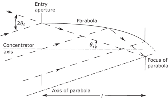
FIGURE 4.10 Construction of the CPC profile from the edge-ray principle, and that the diameter of the entry aperture is

Also, from Equations (4.2) and (4.3) or directly from the figure,

Figure 4.11 shows scale drawing of typical CPCs with a range of collecting angles. It is shown in Appendix C that the concentrator wall has zero slope at the entry aperture, as drawn.

The most remarkable result is Equation (4.3). We see from this that the CPC would have the maximum theoretical concentration ratio (see Section 2.7)

provided all the rays inside the collecting angle 0, actually emerge from the exit aperture. Our use of the edge-ray principle suggests that this ought to be the case, given the analogy with image-forming concentrators, but in fact this is not so. The 3D CPC, like the cone concentrator, has multiple reflections, and these can actually turn back the rays that enter inside the maximum collecting angle. Nevertheless, the transmission-angle curves for CPCs, as calculated by ray-tracing, approach very closely the ideal square shape, of course in practical implementation we usually shorten the length by ~l/3 (called truncation). Figure 4.12, after Winston (1970), shows a typical transmission-angle curve for a CPC with 6j= 16°. It can be seen that the CPC comes very close to being an ideal concentrator. Also, it has the advantages of being a very practical design, easy to make for all wavelengths, since it depends on reflection rather than refraction, and of not requiring any extreme material properties. The only disadvantage is that it is very long compared to its diameter, as can be seen from Equation (4.2). This can

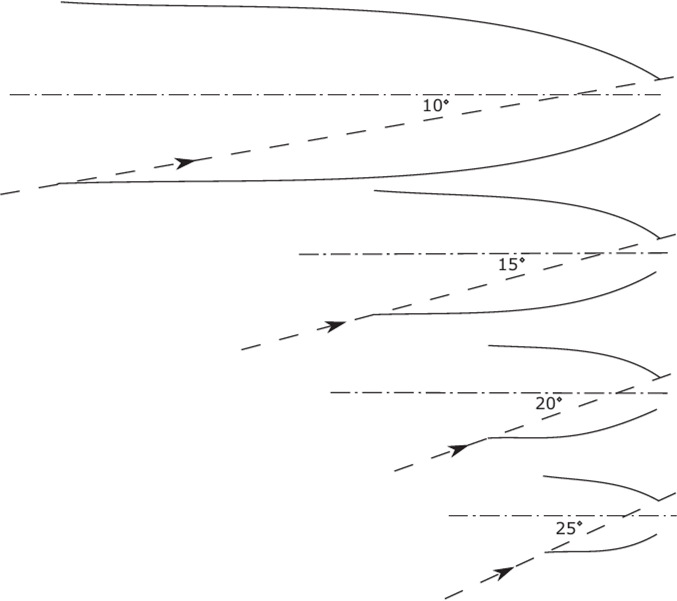
FIGURE 4.11 Some CPCs with different collecting angles. The drawings are to scale with the exit apertures all equal in diameter.

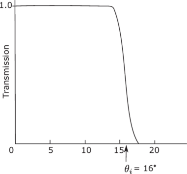
FIGURE 4.12 Transmission-angle curve for a CPC with acceptance angle 9_t= 16°. The cutoff occurs over a range of about 1°.

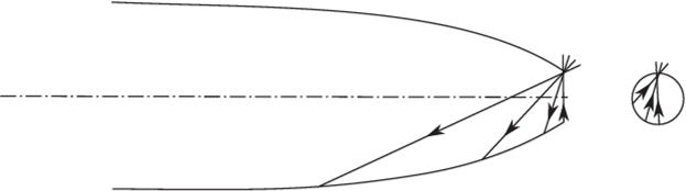
FIGURE 4.13 Identifying rays that are just turned back by a cone like concentrator. The rays shown are intended as projections of skew rays, since the meridional rays through the rim correspond exactly to 0, by construction for a CPC.

be overcome if we incorporate refracting elements into the basic design. In later sections of this chapter we shall study the optics of the CPC in detail. We shall elucidate the mechanism by rays inside the collecting angle which are turned back, give transmission-angle curves for several collecting angles, and give quantitative comparisons with some of the other concentrators, imaging and nonimaging, that have been proposed. In later chapters we shall discuss modifications of the basic CPC along various lines—for example, incorporating transparent refracting materials into the design and even making use of total internal reflection at the walls for all the accepted rays.

We conclude this section by examining the special case of the 2D CPC or trough like a concentrator. This has great practical importance in solar energy applications, since, unlike other trough collectors, it does not require diurnal guiding to follow the sun. The surprising result is obtained that the 2D CPC is actually an ideal concentrator of maximum theoretical concentration ratio—that is, no rays inside the maximum collecting angle are turned back. To show this result we have to find a way of identifying rays that do get turned back after some number of internal reflections. The following procedure for identifying such rays actually applies not only to CPCs but to all axisymmetric cone-like concentrators with internal reflections. It is a way of finding rays on the boundary between sets of rays that are turned back and rays that are transmitted. These extreme rays must just graze the edge of the exit aperture, as in Figure 4.13, so that if we trace rays in reverse from this point in all directions as indicated, these rays appear in the entry aperture on the boundary of the required region. Thus, we could choose a certain input direction, find the reverse traced rays having this direction, and plot their intersections w'ith the plane of the input aperture. They could be sorted according to the number of reflections involved and the boundaries plotted out. Diagrams of this kind will be given for 3D CPCs in the next chapter.

Returning to the 2D CPC, we note first that the ray-tracing in any 2D trough like a reflector is simple even for rays not in a plane perpendicular to the length of the trough. This is because the normal to the surface has no component parallel to the length of the trough, and thus the law of reflection, Equation(2.1), can be applied in two dimensions only. The ray direction cosine in the third dimension is constant. Thus, if Figure 4.14 shows a 2D CPC with the length of the trough perpendicular to the plane of the diagram, all rays can be traced using only their projections on

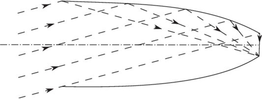
FIGURE 4.14 A 2D CPC. The rays drawn represent projections of rays out of the plane of the diagram.

FIGURE 4.15 The transmission-angle curve for a 2D CPC.

this plane. We can now' apply our identification of rays that get turned back. Since, according to the design, all the rays show'n appear in the entry aperture at 6>_max, there can be no returned rays w'ithin this angle. The 2D CPC has the maximum theoretical concentration ratio and its transmission-angle graph therefore has the ideal shape, as in Figure 4.15^[1]

Since this property is of prime importance, we shall examine the ray paths in more detail to strengthen the verification. Figure 4.16 shows a 2D CPC with a typical ray at the extreme entry angle в_тзх. Say this ray meets the CPC surface at P. A neighboring ray at a smaller angle would be represented by the broken line. There are then two possibilities. Either this ray is transmitted as in the diagram, or else it meets the surface again at PI. In the latter case w'e apply the same argument except using the

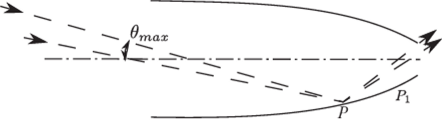
FIGURE 4.16 To prove that a 2D CPC has an ideal transmission-angle characteristic.

extreme ray incident at P1, and so on. Thus, although some rays have a very large number of reflections, eventually they emerge if they entered inside в_пах. Of course, in the preceding argument “ray” includes “projection” of a ray skew to the diagram.

This result shows a difference between 2D and 3D CPCs. The 2D CPC has maximum theoretical concentration, in the sense of Section 2.9. In extending it to 3D, however, we have included more rays (there is now a threefold infinity of rays, allowing for the axial symmetry, whereas in the 2D case we have to consider only a twofold infinity). We have no more degrees of freedom in the design, since the 3D concentrator is obtained from the 2D profile by rotation about the axis of symmetry.

The 3D concentrator has to be a figure of revolution, and thus we can do nothing to ensure that rays outside the meridian sections are properly treated. We shall see in Section 4.7.3 that it is the rays in these regions that are turned back by multiple reflections inside the CPC.

This discussion also shows the different causes of nonideal performance of imaging and nonimaging systems. The rays in an image-forming concentrator such as a high-aperture lens all pass through each surface the same number of times (usually once), and the nonideal performance is caused by geometrical aberrations in the classical sense. In a CPC, on the other hand, different rays have different numbers of reflections before they emerge (or not) at the exit aperture. It is the effect of the reflections in turning back the rays that produces nonideal performance.

Thus, there is an essential difference between a lens with large aberrations and a CPC or other nonimaging concentrator. A CPC is a system of rotational symmetry, and it would be possible to consider all rays as having just, say, three reflections and to discuss the aberrations (no doubt very large) of the image formation by these rays. But there seems no sense in which rays with different numbers of reflections could be said to form an image. It is for this reason that we continue to draw the distinction between image-forming and nonimaging concentrators.

• [1] Strictly, this applies to 2D CPCs that are indefinitely extended along the length of the trough. Inpractice, this effect is achieved by closing the ends with plane mirrors perpendicular to the straightgenerators of the trough. This ensures that all rays entering the rectangular entry aperture w ithin theacceptance angle emerge from the exit aperture.