The Two-Stage CPC

In Section 5.2 we discussed the dielectric-filled CPC using total internal reflection, and we noted that the use of a refractive index greater than unity at the exit aperture permits in principle a greater concentration ratio. In order to utilize this the absorber must be in optical contact with the dielectric, and preferably also the interface must be matched to minimize reflection losses by a suitable coating or a grading of the refractive index. This seems possible, but we then have the practical difficulty that CPCs are very long and therefore a large volume of possibly expensive dielectric is needed. This difficulty may be circumvented by a two-stage system like the one in Figure 5.8. The first stage in air is a (),/(>„ concentrator to give whatever final output angle is needed.

This two-stage system, if designed to give maximum concentration я/sin в, where в is the collecting angle in air, is always longer than a basic CPC designed for concentration 1/sin 0 but with the same collecting aperture. If we make the dielectric part as short as possible—that is, if we maximize в" according to Equation (5.1)— then it can be shown that the overall length of the two-stage system is

FIGURE 5.8 Two-stage system ending in a dielectric of index n. In the diagram, в= 10°, в'= 60°, в"=24.5°, and я = 1.85.

whereas the basic CPC has length

It is easily seen that (5.15) is greater than (5.16). Figure 5.9 shows some typical values for comparison.

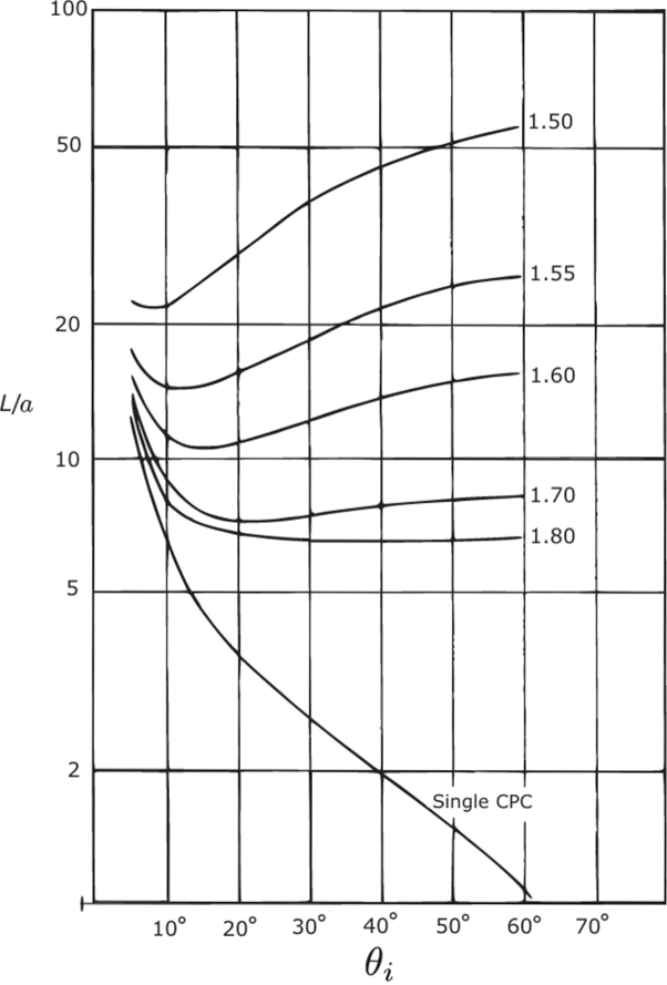
FIGURE 5.9 A comparison of the overall lengths of single- and two-stage concentrators according to Equations (5.15) and (5.16). The ordinate is the ratio of length to radius of collecting aperture, and the graphs are labeled with the refractive index of the second stage.

The CPC Designed for Skew Rays

As we saw in Chapter 4, the basic 3D CPC turns back some skew rays, and this makes its concentration efficiency slightly less than ideal, as shown in Figure 4.15. The basic CPC is designed by applying the edge-ray principle to meridian rays, and this uses up all the degrees of freedom available, so it is not surprising that some skew rays fail. This suggests that we should try designing a concentrator by applying the edge-ray principle to skew rays. The result might then have a slightly closer approach to the maximum theoretical concentration ratio.

Figure 5.10 shows a view from the entry aperture of a concentrator. The entry aperture has a diameter 2a and an exit aperture 2a' = 2a sin 0,. Let this system be designed to fulfill the edge-ray principle for skew rays with skew' invariant h (see Section 2.8). In this projected view a ray enters at 0, and grazes the entry aperture at A, and the exit aperture at В is reflected across to C on the exit aperture (double arrow's). The segment BC is thus tangent to a circle of radius hisin 0,. Another ray AD, also entering at 0„ meets the opposite entry edge at D and is reflected there. In order to satisfy the edge-ray principle, it must meet the edge of the exit aperture and therefore is like the double-arrowed segment AB rotated around the axis so that A reaches D. Thus, the segment reflected from D touches the circle of radius fi/sin (),.

FIGURE 5.10 Design of a concentrator by applying the edge-ray principle to rays with nonzero skew' invariant.

We can show that this segment meets the exit aperture at the same point C as the segment BC reflected at В by calculating the angles subtended at the center by the various ray segments.

The design is completed by requiring that all rays that leave the exit aperture at its rim have entered at the input angle 0,. These rays in the projection of Figure 5.10 are typified by the three-arrowed segments—that is, reflection at some point E along the concentrator to emerge at F on the exit rim. It turns out that the rays do not in general emerge at the same point on the exit rim. Thus, we have a situation where the edge-ray principle is less restrictive than, say, a requirement for imaging at the exit rim. This process completely determines the concentrator as a surface of revolution, but it does not seem to be possible to represent it by any analytical expression. P. Greenman computed the solution for several values of the input angle <9, and skew invariant h. The results are, briefly, that the shapes are very similar to those of the basic CPC for the same 0, but that the overall lengths are less and the transitions in the transmission-angle curves are correspondingly more gradual. Figure 5.11 shows some of these curves.

The overall length of this concentrator is determined, as for the basic CPC, by the extreme rays, as in Figure 5.12. This figure shows the rays ADC and ABC of Figure 5.10, both inclined at the extreme input angle to the axis and both grazing the exit aperture after one and no reflections from the concentrator, respectively. Then in order to admit all rays at 0, or less, the concentrator surface must finish at point A, determined by the intersection of ray ABC with the surface.

This geometry is obvious for the basic CPC, and also in that system the ratio of input to output diameters is set as part of the design data at the desired value 1/ sin 0,. In the present system the design is developed from one end, and it does not follow that the ratio of input to output diameters will have any particular simple value. In fact, it can be shown that this ratio is again 1/sin 0,—a result that is by no means obvious. In spite of this, the concentrator with nonzero h has even less of the maximum theoretical concentration ratio than the basic CPC does, as can be seen by comparing Figures 5.11 and 4.19. This is because the shorter length permits meridian

FIGURE 5.11 Transmission-angle curves for concentrators designed for nonzero skew invariant h. All the concentrators have exit apertures of diameter unity.

FIGURE 5.12 How the length of a concentrator is determined by the extreme rays.

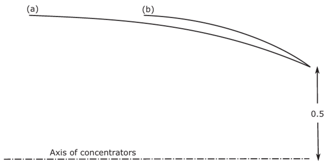
FIGURE 5.13 Comparison of concentrator profiles for 0, =40°; (a) h=0; (b) /;=0.32. It can be seen that meridian rays from the edge of (b) at angles greater than 40° are transmitted, since rays at 40° from the edge of (a) just get through the exit aperture.

rays at angles greater than <9, to reach the exit aperture directly. Thus, by volume conservation of phase space (Appendix A), more rays inside 0, must be rejected.

Figure 5.13 shows a scale-drawing comparison of the basic 40° CPC with concentrators designed for nonzero h. It can be seen how meridian rays at angles greater than в, reach the exit aperture.

The Truncated CPC

A disadvantage of the CPC compared to systems with smaller concentration is that it is very long compared to the diameter of the collecting aperture (or width for 2D systems). This is naturally important for economic reasons in large-scale applications such as solar energy. From Equation (4.2) the length L is approximately equal to the diameter of the collecting aperture divided by the full collecting angle—that is,

If we truncate the CPC by removing part of the entrance aperture end, we find that a considerable reduction in length can be achieved with very little reduction in concentration, so this may be a useful economy.

It is convenient to express the desired relationships in terms of the (г,ф) polar coordinate system as in Figure 5.14. We denote truncated quantities by a subscript T. We are interested in the ratio of the length to the collecting apertures and also in the ratio of the area of the reflector to that of the collecting aperture. We find

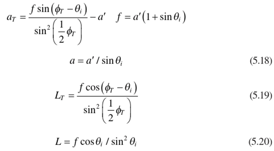
so that

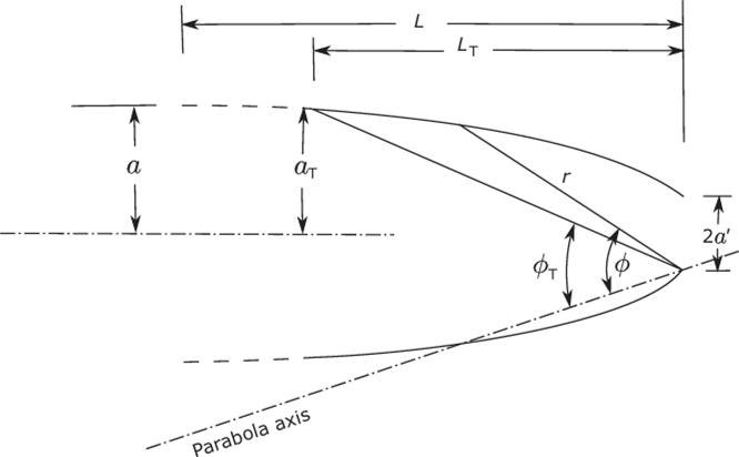
FIGURE 5.14 The polar coordinates used in computing truncation effects.

Plots of this quantity against the theoretical concentration ratio aT/a' for 2D truncated CPCs were given by Rabl (1979) and by Winston and Hinterberger (1975). Figure 5.15 shows some of these curves, and it can be seen that initially—for points near the broken line locus for full CPCs—the curves have a very large slope, so the loss in concentration ratio is quite small for useful truncations.

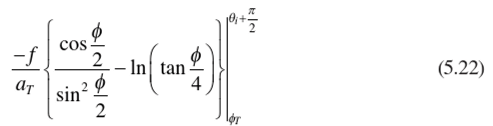
In addition to the ratio of length to aperture diameter w'e may be interested in the ratio of the surface area of reflector to aperture area, since this governs the cost of material for the reflector. The general forms of the curves would be similar to those in Figure 5.15 but with differences between 2D and 3D concentrators. The explicit formulae for reflector area divided by collector area are, for a 2D truncated CPC,

and for a 3D truncated concentrator

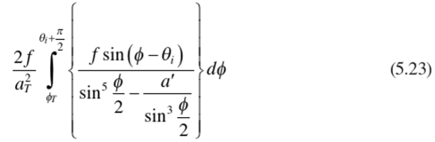
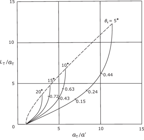
FIGURE 5.15 Length as a function of concentration ratio for 2D truncated concentrators. The numbers marked on the curves are the actual truncation ratios—that is, Z./L.

Derivations of the preceding results and the explicit form of the integral in Equation (5.23) are given in Appendix E. Some representative plots of these functions are given in Figures 5.16 and 5.17. It should be noted that in these figures the theoretical concentration ratios are respectively (aja') and (Ojla')². We conclude from this that losses in performance due to moderate truncation would be acceptable in many instances on account of the economic gains.